From STAC to Data: Accessing EOPF Zarr with xarray

Introduction

In this tutorial we will demonstrate how to access EOPF Zarr products directly from the EOPF Sentinel Zarr Sample Service STAC Catalog.

What we will learn

• ☁️ How to open cloud-optimised datasets from the EOPF Zarr STAC Catalog with xarray
• 🔎 Examing loaded datasets
• 📊 Perform simple data analyses with the loaded data

Prerequisites

This tutorial requires the xarray-eopf extension for data manipulation. To find out more about the library, access the documentation.

It is advised that you go through the previous section, as it gives you an introduction on how to programmatically access a STAC catalog.

---

Import libraries

import requests
import numpy as np
import matplotlib.pyplot as plt
from typing import List, Optional, cast
from pystac import Collection, MediaType
from pystac_client import Client, CollectionClient
from datetime import datetime
import xarray as xr

Helper functions

list_found_elements

As we are expecting to visualise several elements that will be stored in lists, we define a function that will allow us retrieve item id’s and collections id’s for further retrieval.

def list_found_elements(search_result):
    id = []
    coll = []
    for item in search_result.items(): #retrieves the result inside the catalogue.
        id.append(item.id)
        coll.append(item.collection_id)
    return id , coll

---

Establish a connection to the EOPF Zarr STAC Catalog

Our first step is to a connection to the EOPF Zarr STAC Catalog. This involves defining the url of the STAC endpoint. See the previous section for a more detailed explanation how to retrieve the enpoint URL.

Through the Client.open() function, we can establish the connection to the EOPF Zarr STAC catalog by providing the specific url.

max_description_length = 100

eopf_stac_api_root_endpoint = "https://stac.core.eopf.eodc.eu/" #root starting point
eopf_catalog = Client.open(url=eopf_stac_api_root_endpoint)
# eopf_catalog  #print to have an interative visualisation

Filtering for items of interest

For this tutorial, we will focus on the Sentinel-2 L2A Collection. The EOPF STAC Catalog corresponding id is: sentinel-2-l2a.

As we are interested in retrieving and exploring an Item from the collection, we will focus again over the Innsbruck area we have defined in the previous tutorial.

innsbruck_s2 = eopf_catalog.search( # searching in the Catalog
    collections= 'sentinel-2-l2a', # interest Collection,
    bbox=(11.124756, 47.311058, # AOI extent
          11.459839,47.463624),
    datetime='2020-05-01T00:00:00Z/2025-05-31T23:59:59.999999Z' # interest period
)

combined_ins =list_found_elements(innsbruck_s2)

print("Search Results:")
print('Total Items Found for Sentinel-2 L-2A over Innsbruck:  ',len(combined_ins[0]))

Search Results:
Total Items Found for Sentinel-2 L-2A over Innsbruck:   27

Let us now select the first Item in the list of 27 Items.

first_item_id=combined_ins[0][0]
print(first_item_id)

S2B_MSIL2A_20250530T101559_N0511_R065_T32TPT_20250530T130924

In a next step, we retrieve the URL of the cloud location for the specific item. We will need the url to access and load the selected Item with the help of xarray.

c_sentinel2 = eopf_catalog.get_collection('sentinel-2-l2a')
#Choosing the first item available to be opened:
item= c_sentinel2.get_item(id=first_item_id)
item_assets = item.get_assets(media_type=MediaType.ZARR)

cloud_storage = item_assets['product'].href

print('Item cloud storage URL for retrieval:',cloud_storage)

Item cloud storage URL for retrieval: https://objects.eodc.eu:443/e05ab01a9d56408d82ac32d69a5aae2a:202505-s02msil2a/30/products/cpm_v256/S2B_MSIL2A_20250530T101559_N0511_R065_T32TPT_20250530T130924.zarr

Examining Dataset Structure

In the following step, we open the cloud-optimised Zarr dataset using xarray.open_datatree supported by the xarray-eopf extension.

The subsequent loop then prints out all the available groups within the opened DataTree, providing a comprehensive overview of the hierarchical structure of the EOPF Zarr products.

dt = xr.open_datatree(
    cloud_storage,        # the cloud storage url from the Item we are interested in
    engine="eopf-zarr",   # xarray-eopf defined engine 
    op_mode="native",     # visualisation mode
    chunks={})            # default eopf chunking size

for dt_group in sorted(dt.groups):
    print("DataTree group {group_name}".format(group_name=dt_group)) # getting the available groups

DataTree group /
DataTree group /conditions
DataTree group /conditions/geometry
DataTree group /conditions/mask
DataTree group /conditions/mask/detector_footprint
DataTree group /conditions/mask/detector_footprint/r10m
DataTree group /conditions/mask/detector_footprint/r20m
DataTree group /conditions/mask/detector_footprint/r60m
DataTree group /conditions/mask/l1c_classification
DataTree group /conditions/mask/l1c_classification/r60m
DataTree group /conditions/mask/l2a_classification
DataTree group /conditions/mask/l2a_classification/r20m
DataTree group /conditions/mask/l2a_classification/r60m
DataTree group /conditions/meteorology
DataTree group /conditions/meteorology/cams
DataTree group /conditions/meteorology/ecmwf
DataTree group /measurements
DataTree group /measurements/reflectance
DataTree group /measurements/reflectance/r10m
DataTree group /measurements/reflectance/r20m
DataTree group /measurements/reflectance/r60m
DataTree group /quality
DataTree group /quality/atmosphere
DataTree group /quality/atmosphere/r10m
DataTree group /quality/atmosphere/r20m
DataTree group /quality/atmosphere/r60m
DataTree group /quality/l2a_quicklook
DataTree group /quality/l2a_quicklook/r10m
DataTree group /quality/l2a_quicklook/r20m
DataTree group /quality/l2a_quicklook/r60m
DataTree group /quality/mask
DataTree group /quality/mask/r10m
DataTree group /quality/mask/r20m
DataTree group /quality/mask/r60m
DataTree group /quality/probability
DataTree group /quality/probability/r20m

Root Dataset Metadata

We specifically look for groups containing data variables under /measurements/reflectance/r20m (which corresponds to Sentinel-2 bands at 20m resolution). The output provides key information about the selected group, including its dimensions, available data variables (the different spectral bands), and coordinates.

# Get /measurements/reflectance/r20m group
groups = list(dt.groups)
interesting_groups = [
    group for group in groups if group.startswith('/measurements/reflectance/r20m')
    and dt[group].ds.data_vars
]
print(f"\n🔍 Searching for groups with data variables in '/measurements/reflectance/r20m'...")

🔍 Searching for groups with data variables in '/measurements/reflectance/r20m'...

if interesting_groups:
    sample_group = interesting_groups[0]
    group_ds = dt[sample_group].ds
    
    print(f"Group '{sample_group}' Information")
    print("=" * 50)
    print(f"Dimensions: {dict(group_ds.dims)}")
    print(f"Data Variables: {list(group_ds.data_vars.keys())}")
    print(f"Coordinates: {list(group_ds.coords.keys())}")

else:
    print("No groups with data variables found in the first 5 groups.")

Group '/measurements/reflectance/r20m' Information
==================================================
Dimensions: {'y': 5490, 'x': 5490}
Data Variables: ['b01', 'b02', 'b03', 'b04', 'b05', 'b06', 'b07', 'b11', 'b12', 'b8a']
Coordinates: ['x', 'y']

/tmp/ipykernel_1128780/1451209294.py:7: FutureWarning: The return type of `Dataset.dims` will be changed to return a set of dimension names in future, in order to be more consistent with `DataArray.dims`. To access a mapping from dimension names to lengths, please use `Dataset.sizes`.
  print(f"Dimensions: {dict(group_ds.dims)}")

In a next step, we inspect the attributes of the root dataset within the DataTree. Attributes often contain important high-level metadata about the entire product, such as processing details, STAC discovery information, and more. We print the first few attributes to get an idea of the available metadata.

# Examine the root dataset
root_dataset = dt.ds

print("Root Dataset Metadata")

if root_dataset.attrs:
    print(f"\nAttributes (first 3):")
    for key, value in list(root_dataset.attrs.items())[:3]:
        print(f"   {key}: {str(value)[:80]}{'...' if len(str(value)) > 80 else ''}")

Root Dataset Metadata

Attributes (first 3):
   other_metadata: {'AOT_retrieval_model': 'SEN2COR_DDV', 'L0_ancillary_data_quality': '4', 'L0_eph...
   stac_discovery: {'assets': {'analytic': {'eo:bands': [{'center_wavelength': 0.4423, 'common_name...

Visualising the RGB quicklook composite

EOPF Zarr Assets include a quicklook RGB composite, which we now want to open and visuliase. We open the Zarr dataset again, but this time, we specifically target the quality/l2a_quicklook/r20m group and its variables.

This group typically contains a true-colour (RGB) quicklook composite, which is a readily viewable representation of the satellite image.

We use xr.open_dataset() and specify the following set of arguments in order to load the quicklook.

## Visualising the RGB quicklook composite:
ds = xr.open_dataset(
    cloud_storage,        # the cloud storage url from the Item we are interested in
    engine="eopf-zarr",   # xarray-eopf defined engine 
    op_mode="native",     # visualisation mode
    chunks={},            # default eopf chunking size
    group_sep="/",
    variables="quality/l2a_quicklook/r20m/*",
)

As soon as we loaded it, we can create a simple plot with imshow() to see the quicklook.

ds["quality/l2a_quicklook/r20m/tci"].plot.imshow()
plt.title('RGB Quicklook')
plt.xlabel('X-coordinate')
plt.ylabel('Y-coordinate')
plt.grid(False) # Turn off grid for image plots
plt.axis('tight') # Ensure axes fit the data tightly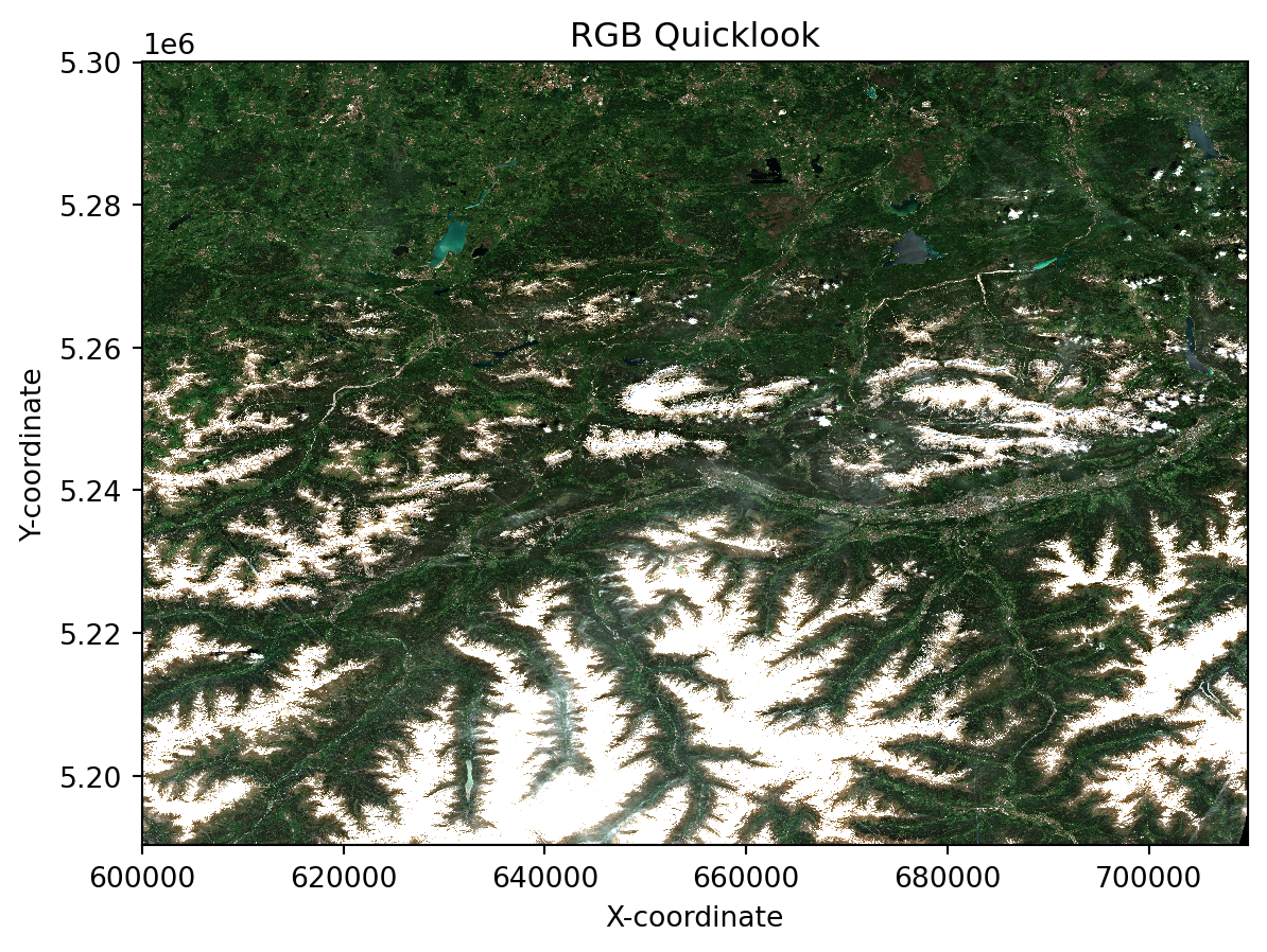

Simple Data Analysis: Calculating NDVI

Let us now do a simple analysis with the data from the EOPF Zarr STAC Catalog. Let us calculate the Normalized Difference Vegetation Index (NDVI).

First, we open the Zarr dataset specifically for the red (B04) and Near-Infrared (B08) bands, which are crucial for the calculation of the NDVI. We also specify resolution=20 to ensure we are working with the 20-meter resolution bands.

red_nir = xr.open_dataset(
    cloud_storage,
    engine="eopf-zarr",
    chunks={},
    spline_orders=0,
    variables=['b04', 'b08'],
    resolution= 60,
)

In a next step, we cast the red (B04) and Near-Infrared (B08) bands to floating-point numbers. This is important for accurate mathematical operations, which we will conduct in the next cell.

red_f = red_nir.b04.astype(float)
nir_f = red_nir.b08.astype(float)

Now, we perform the initial steps for NDVI calculation: - sum_bands: Calculates the sum of the Near-Infrared and Red bands. - diff_bands: Calculates the difference between the Near-Infrared and Red bands.

sum_bands = nir_f + red_f
diff_bands = nir_f - red_f
ndvi = diff_bands / sum_bands

To prevent division by zero errors in areas where both red and NIR bands might be zero (e.g., water bodies or clouds), this line replaces any NaN values resulting from division by zero with 0. This ensures a clean and robust NDVI product.

ndvi = ndvi.where(sum_bands != 0, 0)

In a final step, we can visualise the calculated NDVI.

ndvi.plot(cmap='RdYlGn', vmin=-1, vmax=1)
plt.title('Normalized Difference Vegetation Index (NDVI)')
plt.xlabel('X-coordinate')
plt.ylabel('Y-coordinate')
plt.grid(False) # Turn off grid for image plots
plt.axis('tight') # Ensure axes fit the data tightly

# Display the plot
plt.show()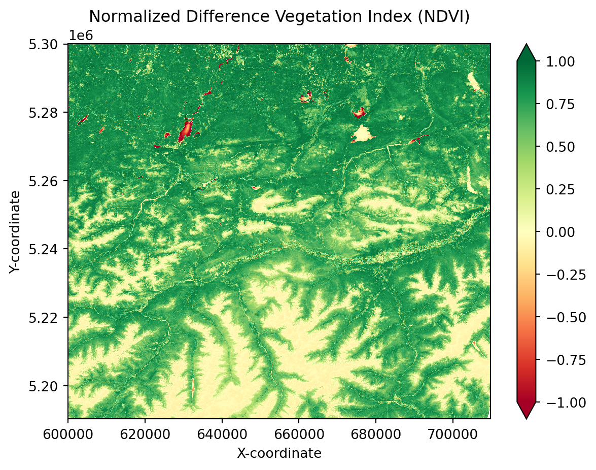

💪 Now it is your turn

With the foundations learned so far, you are now equipped to access products from the EOPF Zarr STAC catalog. These are your tasks: ### Task 1: Explore five additional Sentinel-2 Items for Innsbruck Replicate the RGB quicklook and have an overview of the spatial changes.

Task 2: Calculate NDVI

Replicate the NDVI calculation for the additional Innsbruck items.

Task 3: Applying more advanced analysis techniques

The EOPF STAC Catalog offers a wealth of data beyond Sentinel-2. Replicate the search and data access for data from other collections.

Conclusion

In this section we established a connection to the EOPF Sentinel Zarr Sample Service STAC Catalog and directly accessed an EOPF Zarr item with xarray. In the tutorial you are guided through the process of opening hierarchical EOPF Zarr products using xarray’s DataTree, a library designed for accessing complex hierarchical data structures.

What’s next?

This online resource is under active development. So stay tuned for regular updates.