import xarray as xr
import numpy as np
import pandas as pd

import matplotlib.pyplot as plt

import dask
import spyndex

from dask.distributed import ClientAnalyzing Forest Vegetation Anomalies Using Sentinel-2 Zarr Data Cubes
By: @davemlz | InfAI Infinity GmbH
Introduction
Forests are the largest terrestrial carbon sinks, playing a critical role in regulating the global carbon cycle through sustained CO\(_2\) uptake. However, extreme climate events (such as heatwaves and droughts) can disrupt forest functioning, reducing photosynthetic activity and, in severe cases, causing tree mortality.
While in situ measurements provide valuable information on forest health, collecting such data over large areas is costly, time-consuming, and logistically challenging. Scalable and continuous monitoring therefore requires more efficient approaches.
In this case study, we will explore how to use Sentinel-2 L2A data stored as Zarr data cubes to analyze vegetation anomalies in forest ecosystems in Germany. Specifically, we will focus on two ICOS sites affected by the drought of 2018: DE-Hai and DE-Tha, with DE-Tha left for learners to explore on their own.
By leveraging spatiotemporal data cubes, we will compute spectral indices and derive anomaly time series to evaluate forest responses to extreme events in CO\(_2\) uptake (Gross Primary Production, GPP, from ICOS). This notebook will guide you through a modular workflow for:
- Accessing Sentinel-2 Zarr data from STAC.
- Calculating vegetation indices.
- Detecting anomalies in time series.
- Visualizing forest responses to environmental extremes.
Through this study case, you will see the potential of Zarr-based data cubes for scalable forest monitoring.
What we will learn
In this notebook, you will gain hands-on experience with the following:
- 🚀 Creating Sentinel-2 L2A data cubes from the EOPF Zarr STAC.
- 🔎 Operating on data cubes, including resampling and interpolation.
- 🌿 Computing spectral indices using Awesome Spectral Indices.
- 📈 Deriving vegetation anomalies from time series data.
- 📊 Visualizing time series and comparing results against GPP measurements from ICOS.
Prerequisites
To analyze vegetation anomalies, we will work with vegetation indices. To leverage the full power of xarray, we will use the spyndex Python package, which provides a Python API for the Awesome Spectral Indices catalogue. This gives access to over 200 spectral indices, which can be computed directly on various Python data types, including xarray datasets and data arrays.
For more details, refer to the Awesome Spectral Indices paper in Scientific Data.
Import libraries
Helper functions
Helper functions were defined in the vegetation_anomalies_utils.py file. Here we import all of the functions and explain their role.
from vegetation_anomalies_utils import *get_items
This function queries the EOPF STAC API for Sentinel-2 L2A items that intersect a specified latitude/longitude point within a given date range.
latlon_to_buffer_bbox
This function converts a latitude/longitude point to a specified projected coordinate system (EPSG) and then generates a square bounding box centered on that point.
This helper is not used directly as it is incorporated in the next helper function.
open_and_curate_data
This function opens a Sentinel-2 STAC item (Zarr), performs a spatial subset around a given point, applies SCL-based masking, and returns an xarray.Dataset containing only the selected reflectance bands (e.g. B04, B8A) with a time dimension. It uses the validate_scl function from Zarr_wf_utils.py.
Note: This function is a delayed Dask object, meaning it will only be executed when explicitly triggered through Dask.
curate_gpp
This function loads a GPP time series, computes weekly anomalies, identifies extreme low-GPP events, and filters these extremes to retain only events lasting at least a specified number of consecutive weeks.
Vegetation Anomalies in the Hainich National Park
We will start the notebook with a forest ecosystem that was severely affacted by the drought of 2018: DE-Hai.
# DE-Hai Coordinates
HAI_LAT = 51.079212
HAI_LON = 10.452168
Initialize a Dask distributed client to enable parallel and delayed computation. This will manage the execution of tasks, such as loading and processing large Sentinel-2 Zarr datasets, efficiently.
client = Client()
client
Client
Client-6ae3d25b-68a3-11f1-8e3c-6e9a916ac8c0
| Connection method: Cluster object | Cluster type: distributed.LocalCluster |
| Dashboard: http://127.0.0.1:8787/status |
Cluster Info
LocalCluster
617537e9
| Dashboard: http://127.0.0.1:8787/status | Workers: 4 |
| Total threads: 8 | Total memory: 31.34 GiB |
| Status: running | Using processes: True |
Scheduler Info
Scheduler
Scheduler-47aa6226-fee9-4d2c-8e7b-cea8745192f4
| Comm: tcp://127.0.0.1:45579 | Workers: 0 |
| Dashboard: http://127.0.0.1:8787/status | Total threads: 0 |
| Started: Just now | Total memory: 0 B |
Workers
Worker: 0
| Comm: tcp://127.0.0.1:35039 | Total threads: 2 |
| Dashboard: http://127.0.0.1:41779/status | Memory: 7.84 GiB |
| Nanny: tcp://127.0.0.1:36583 | |
| Local directory: /tmp/dask-scratch-space/worker-t42ufiel | |
Worker: 1
| Comm: tcp://127.0.0.1:39489 | Total threads: 2 |
| Dashboard: http://127.0.0.1:43099/status | Memory: 7.84 GiB |
| Nanny: tcp://127.0.0.1:34773 | |
| Local directory: /tmp/dask-scratch-space/worker-m80srlmt | |
Worker: 2
| Comm: tcp://127.0.0.1:41447 | Total threads: 2 |
| Dashboard: http://127.0.0.1:35313/status | Memory: 7.84 GiB |
| Nanny: tcp://127.0.0.1:37763 | |
| Local directory: /tmp/dask-scratch-space/worker-js35rrp7 | |
Worker: 3
| Comm: tcp://127.0.0.1:36107 | Total threads: 2 |
| Dashboard: http://127.0.0.1:42057/status | Memory: 7.84 GiB |
| Nanny: tcp://127.0.0.1:35261 | |
| Local directory: /tmp/dask-scratch-space/worker-fcbguql2 | |
Load the GPP data
Load the GPP time series for the DE-Hai site and compute weekly anomalies, identifying extreme low-GPP events.
- The following helper function just needs one of two possible inputs: “DE-Hai” (this example), or “DE-Tha” (for learners to explore).
The obtained dataframe contains the following columns:
GPP_NT_VUT_REF: Gross Primary Production (GPP) values per week.weekofyear: Number of the week of the year [1-53].anomaly: GPP anomalies, computed as the deviation from the mean seasonal cycle.extreme: Whether the specific value was a extreme or not (1 = extreme, 0 = normal).
HAI_df = curate_gpp("DE-Hai")Create the Sentinel-2 L2A Data Cube
First, query the EOPF STAC API to retrieve Sentinel-2 L2A items for the DE-Hai site.
- We specify for the following helper function the coordinates of the site (
lat,lon), and we setreturn_as_dictsto True to avoid ocnflicts when a href link is not present in an asset of the retrieved items.
# Get all items as a list of dicts
HAI_items = get_items(HAI_LAT,HAI_LON,return_as_dicts=True)
For each item, open and curate the data by subsetting around the site coordinates and selecting the relevant bands:
- The
itemparameter is a dictionary obtained from each item inHAI_items. - We specify the coordinates of the site (
lat,lon). - The
bandsparameter is a list of the bands you want to retrive, in this case we just want the red and near-infrared bands (b04 and b8a). - The
resolutionwe will use is 20 m: This must be one of 10, 20 or 60. - The
bufferparameter us set to 500 m (a bounding box is constructed from this parameter as well as from thelat,lonparameters). - Finally,
items_as_dictsis set to True since we defined it in the previous code cell.
After this, datasets are computed in parallel with Dask.
# Create the delayed Dask objects
HAI_ds = [open_and_curate_data(item,lat=HAI_LAT,lon=HAI_LON,bands=["b04","b8a"],resolution=20,buffer=500,items_as_dicts=True) for item in HAI_items]

# Compute the delayed objects in parallel. This outputs a list of xarray.Dataset objects
HAI_data = dask.compute(*HAI_ds)
After computed, datasets are concatenated along the time dimension, sorted by time, and finally loaded into memory as a single xarray.Dataset.
# Concatenate the previous list using the time dimension and sort it
HAI_ds = xr.concat(HAI_data,dim="time").sortby("time")

# Load it into memory
HAI_ds = HAI_ds.compute()
Compute Vegetation Indices
Compute spectral indices for the DE-Hai dataset using the spyndex package. In this example, we calculate NDVI and kernel NDVI (kNDVI).
- NDVI (Normalized Difference Vegetation Index) is a widely used index to monitor vegetation health and greenness. It is calculated as:
\[\text{NDVI} = \frac{N - R}{N + R}\]
where N is the near-infrared band (B8A) and R is the red band (B04).
- kNDVI (Kernel NDVI) is a kernelized version of NDVI. Here, an RBF (Radial Basis Function) kernel is applied:
\[\text{kNDVI} = \frac{k(N,N) - k(N,R)}{k(N,N) + k(N,R)}\]
where \(k(a,b)\) is the RBF kernel:
\[k(N,N) = 1\]
\[k(N,R) = \exp\left(-\frac{(N-R)^2}{2 \sigma^2}\right)\]
Here, \(\sigma\) is claculated as the median in the time dimension of \(0.5(N+R)\).
The spyndex.computeIndex function computes both indices across the time series and stores them in an xarray.Dataset named idx for subsequent anomaly analysis.
The spyndex.computeKernel function computes the kernel for the kNDVI.
Note that in both cases spyndex just requires the data for computing the indices without the need of hard-coding the formulas.
idx = spyndex.computeIndex(
    ["NDVI","kNDVI"], # Indices to compute
    N = HAI_ds["b8a"], # NIR band
    R = HAI_ds["b04"], # Red band
    kNN = 1.0,
    kNR = spyndex.computeKernel(
        "RBF", # RBF kernel
        a = HAI_ds["b8a"],
        b = HAI_ds["b04"],
        sigma = ((HAI_ds["b8a"] + HAI_ds["b04"])/2.0).median("time")
    )
).to_dataset("index")
Add the name and units of each index to the attributes according to the CF conventions.
idx.NDVI.attrs["long_name"] = spyndex.indices.NDVI.long_name
idx.NDVI.attrs["units"] = "1"

idx.kNDVI.attrs["long_name"] = spyndex.indices.kNDVI.long_name
idx.kNDVI.attrs["units"] = "1"
Resample the NDVI and kNDVI time series to weekly frequency, taking the median within each week. After resampling, fill temporal gaps by applying cubic interpolation along the time dimension. This produces smooth, continuous weekly index time series suitable for anomaly computation.
idx = idx.resample(time="1W").median().interpolate_na(dim="time",method="cubic")Calculate Vegetation Anomalies
Compute the median seasonal cycle (MSC) for NDVI and kNDVI.
By grouping the time series by weekofyear and taking the median across years, this step produces a climatological baseline that represents the typical vegetation state for each week of the year.
The MSC will be used later to derive vegetation anomalies.
msc = idx.groupby("time.weekofyear").median("time")Plot the MSC of the NDVI.
msc.NDVI.plot.imshow(col = "weekofyear",cmap = "viridis",col_wrap = 8,vmin=0,vmax=1)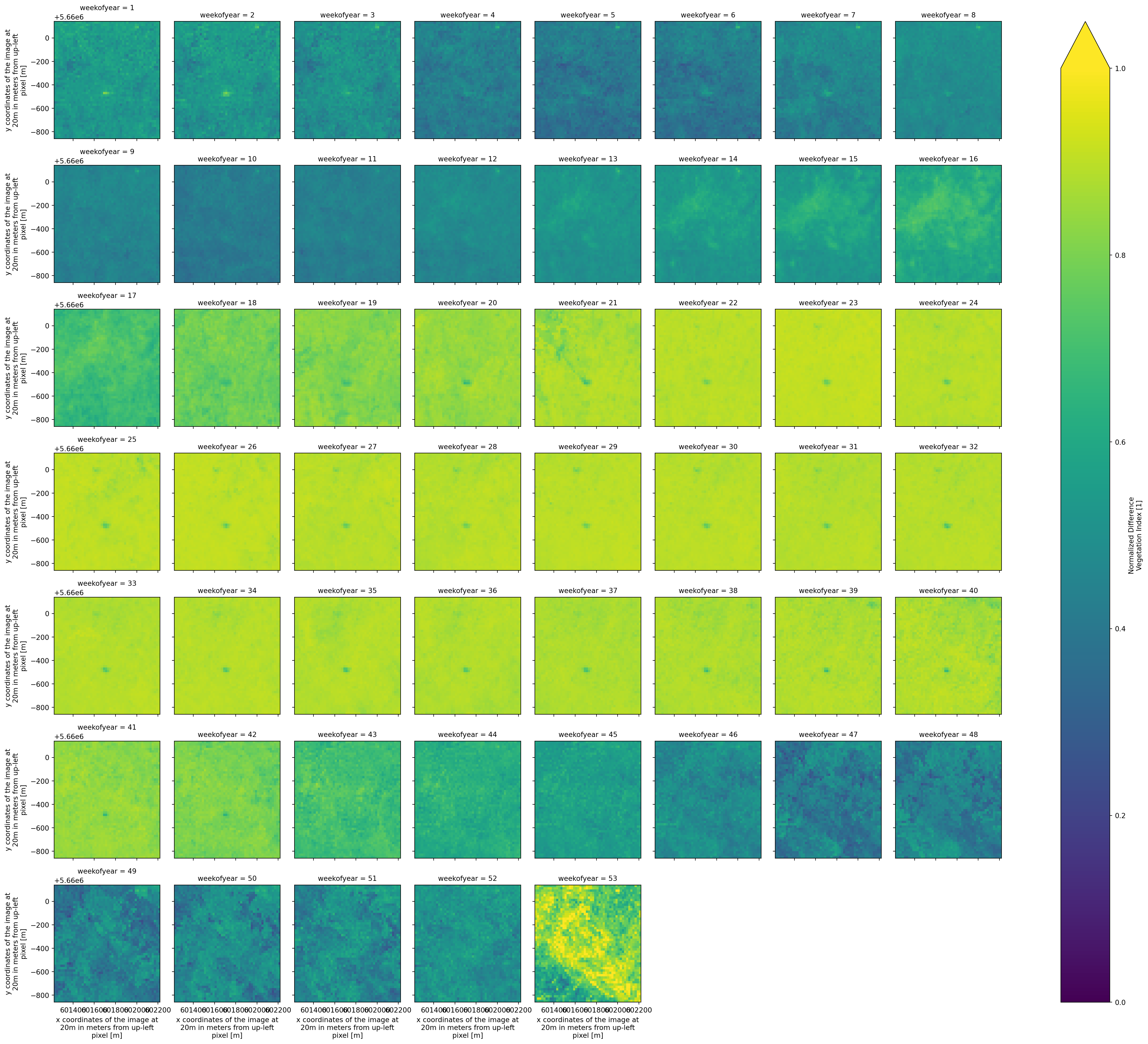
Plot the MSC of the kNDVI.
msc.kNDVI.plot.imshow(col = "weekofyear",cmap = "viridis",col_wrap = 8,vmin=0,vmax=1)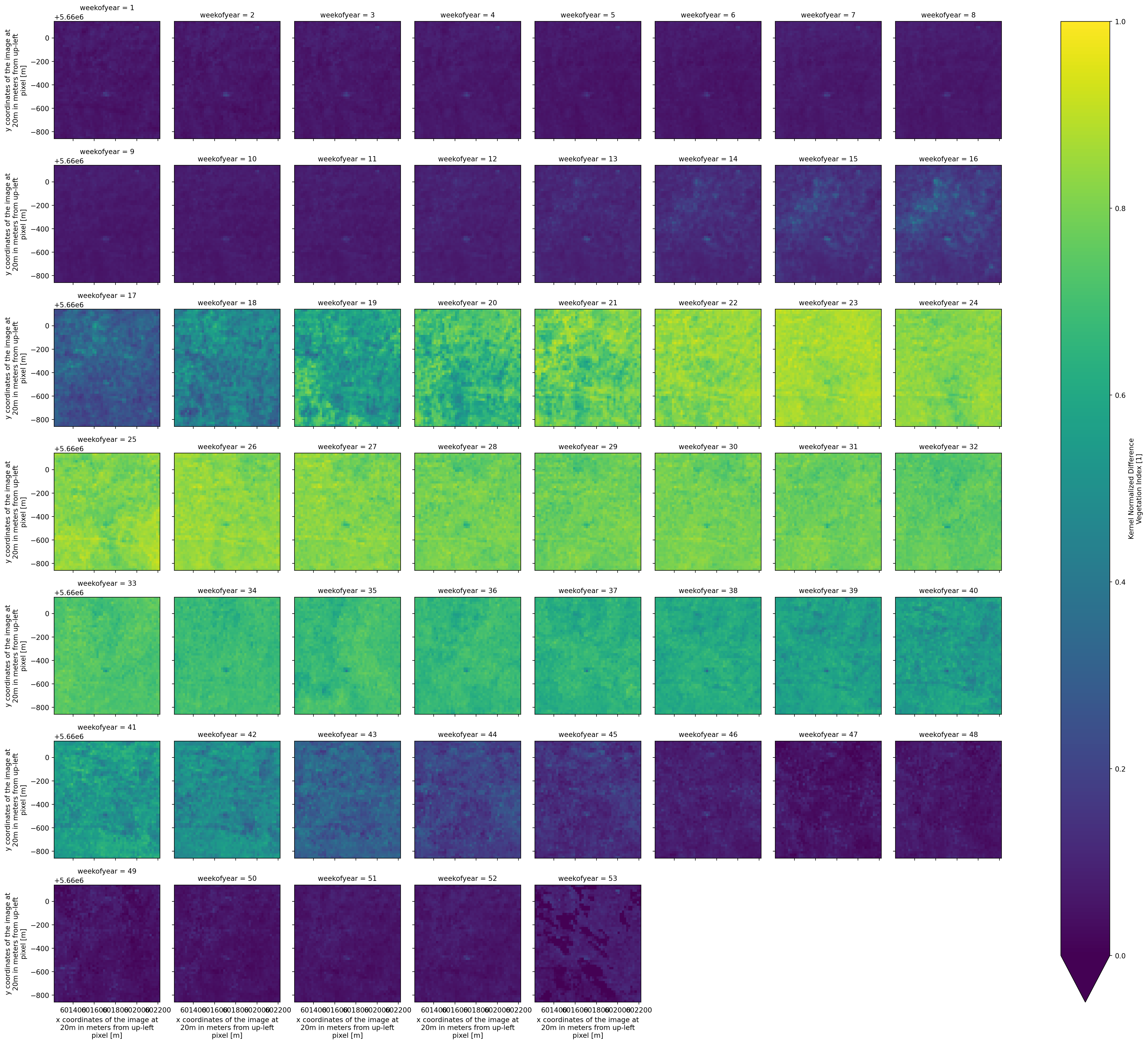
Compute vegetation anomalies by subtracting the median seasonal cycle (MSC) from the weekly NDVI and kNDVI values. This step isolates deviations from the expected seasonal pattern, allowing us to identify abnormal vegetation conditions potentially linked to stress or extreme events.
idx_anomalies = idx.groupby("time.weekofyear") - mscAdd the name and units of each index anomaly to the attributes according to the CF conventions.
idx_anomalies.NDVI.attrs["long_name"] = spyndex.indices.NDVI.long_name + " Anomaly"
idx_anomalies.NDVI.attrs["units"] = "1"

idx_anomalies.kNDVI.attrs["long_name"] = spyndex.indices.kNDVI.long_name + " Anomaly"
idx_anomalies.kNDVI.attrs["units"] = "1"
Visualize Time Series
We will use time series for visualization. Let’s first aggregate the indices in space using the median to produce a time series.
idx_agg = idx.median(["x","y"])Here, we defined the colors to use for our indices.
# Colors for indices
NDVI_COLOR = 'limegreen'
kNDVI_COLOR = 'darkviolet'

# Color for zero line in anomalies
ZERO_COLOR = 'red'
Now, we will plot the NDVI and kNDVI time series together with the GPP measurements for the DE-Hai site. A secondary axis will be used to display GPP, allowing direct visual comparison between vegetation dynamics and ecosystem productivity. Extreme low-GPP events are highlighted as shaded red intervals: These events are defined as periods of at least two consecutive days in which GPP anomalies fall below the 10th percentile of the lower tail of the distribution. This information is contained in the HAI_df dataframe created via curate_gpp helper function.
This visualization helps link vegetation index to observed reductions in carbon uptake, revealing how forest canopy responses relate to ecosystem-scale stress signals.
fig, ax = plt.subplots(figsize=(15, 3))

ax.plot(idx_agg.time, idx_agg["NDVI"],  color=NDVI_COLOR,  label="NDVI")
ax.plot(idx_agg.time, idx_agg["kNDVI"], color=kNDVI_COLOR, label="kNDVI")
ax.set_ylim([-0.15,1.2])
ax.set_ylabel("VI")
ax.legend(loc="upper left")

ax2 = ax.twinx()
ax2.scatter(HAI_df.index, HAI_df["GPP_NT_VUT_REF"],
            s=20, color="grey", alpha=0.6, label="GPP")
ax2.set_ylim([-3.5,17.5])
ax2.set_ylabel("GPP")
ax2.legend(loc="upper right")

extreme_mask = HAI_df["extreme"] == 1
groups = (extreme_mask != extreme_mask.shift()).cumsum()

for _, group in HAI_df[extreme_mask].groupby(groups):
    start = group.index.min()
    end   = group.index.max()
    ax.axvspan(start, end, color="red", alpha=0.15)

plt.title("NDVI, kNDVI, GPP and Extreme Events")
plt.tight_layout()
plt.show()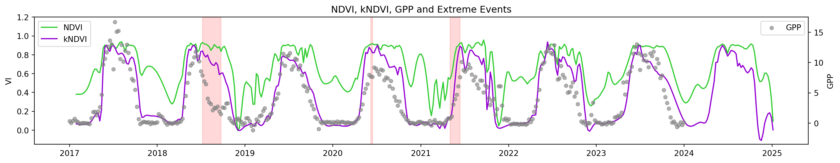
Now, let’s do the same for the anomalies by aggregating the anomalies of the indices in space using the median to produce a time series.
idx_anomalies_agg = idx_anomalies.median(["x","y"])Now we can visualize the anomaly time series of NDVI, kNDVI, and GPP for the DE-Hai site. Here, both vegetation indices and GPP have been transformed into weekly anomalies, representing deviations from their typical seasonal cycles. A horizontal line at zero indicates the expected baseline. A secondary axis displays GPP anomalies, allowing direct comparison between canopy-level spectral responses and ecosystem-level carbon uptake changes. Extreme low-GPP events are shown as shaded red intervals.
This plot highlights how vegetation index anomalies co-occur with (e.g. 2021) or diverge (e.g. 2018) from carbon uptake anomalies, offering insight into forest responses to stress events.
fig, ax = plt.subplots(figsize=(15, 3))

ax.plot(idx_anomalies_agg.time, idx_anomalies_agg["NDVI"],  color=NDVI_COLOR,  label="NDVI")
ax.plot(idx_anomalies_agg.time, idx_anomalies_agg["kNDVI"], color=kNDVI_COLOR, label="kNDVI")
ax.axhline(0, color=ZERO_COLOR, linewidth=1)
ax.set_ylim([-0.45,0.45])
ax.set_ylabel("VI Anomaly")
ax.legend(loc="upper left")

ax2 = ax.twinx()
ax2.scatter(HAI_df.index, HAI_df["anomaly"],
            s=20, color="grey", alpha=0.6, label="GPP")
ax2.set_ylim([-6.5,6.5])
ax2.set_ylabel("GPP Anomaly")
ax2.legend(loc="upper right")

extreme_mask = HAI_df["extreme"] == 1
groups = (extreme_mask != extreme_mask.shift()).cumsum()

for _, group in HAI_df[extreme_mask].groupby(groups):
    start = group.index.min()
    end   = group.index.max()
    ax.axvspan(start, end, color="red", alpha=0.15)

plt.title("NDVI, kNDVI, GPP Anomalies and Extreme Events")
plt.tight_layout()
plt.show()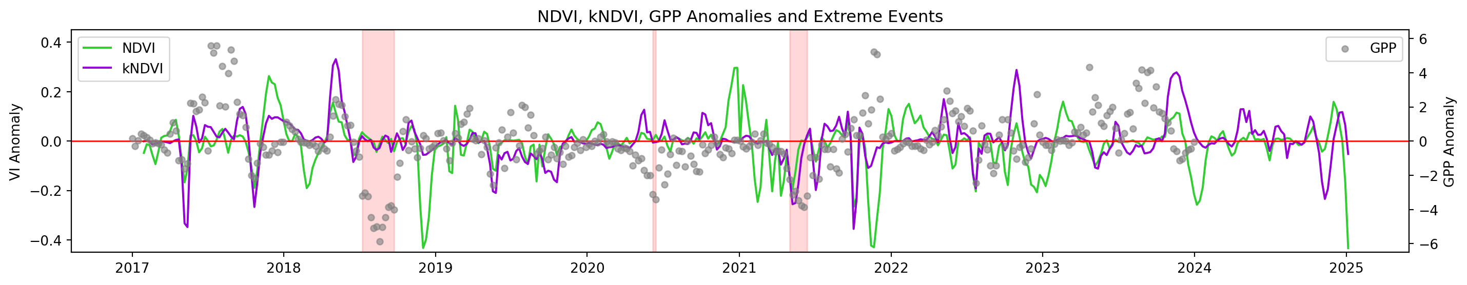
💪 Now it is your turn
The following exercises will help you reproduce the previous workflow for another dataset.
Task 1: Create a data cube for DE-Tha
- Use the coordinates of DE-Tha (provided in the cell below) to create a data cube for this site.
- Retrieve the red edge bands in addition to the NIR and red bands.
- Modify the code as you need.
# DE-Tha Coordinates
THA_LAT = 50.9625
THA_LON = 13.56515

# Get all items as a list of dicts
# THA_items = get_items(THA_LAT,THA_LON,return_as_dicts=True)

# Create the delayed Dask objects
# THA_ds = [open_and_curate_data(..., bands=["b04", "b05", "b06", "b07", "b8a"]) for ...]

# ...
Task 2: Compute Vegetation Indices
- Select a vegetation index from Awesome Spectral Indices that uses the Red Edge bands.
- Modify the code as you need.
# Indices that include any of the red edge bands
for idx, attrs in spyndex.indices.items():
    if any(item in ["RE1","RE2","RE3"] for item in attrs.bands):
        print(idx)
ARI
ARI2
BAIS2
CIRE
CRI700
FDI
GM1
GM2
IRECI
MCARI
MCARI705
MCARIOSAVI
MCARIOSAVI705
MSR705
MTCI
ND705
NDCI
NDREI
NDTI4RE
NDVI4RE
NDVI705
NHFD
PSRI
REDSI
RENDVI
RVI
RVI4RE
S2REP
S2WI
SAVI4RE
SNDTI4RE
SR3
SR555
SR705
STI4RE
SeLI
TCARI
TCARIOSAVI
TCARIOSAVI705
TCI
TRRVI
TTVI
TWI
VARI700
VI700
mND705
mSR705Task 3: Calculate Vegetation Anomalies
- Calculate anomalies for the selected index and compare them against the GPP anomalies of DE-Tha.
THA_df = curate_gpp("DE-Tha")

# THA_df["GPP_NT_VUT_REF"] -> GPP values
# THA_df["time"] -> time simension
# THA_df["anomaly"] -> Anomalies
# THA_df["extreme"] -> Extreme = 1, Normal condition = 0
Conclusion
In this notebook, we explored how Sentinel-2 L2A Zarr data cubes can be used to monitor forest vegetation dynamics and detect anomalous behavior linked to ecosystem stress. By leveraging Zarr, STAC-based discovery, and xarray/Dask for scalable computation, we built an end-to-end workflow that included:
- Accessing Sentinel-2 data from the EOPF Zarr STAC
- Creating spatiotemporal data cubes centered on forest monitoring sites
- Computing spectral indices (NDVI, kNDVI) using the Awesome Spectral Indices catalogue
- Constructing weekly time series and climatological baselines
- Deriving vegetation anomalies and comparing them with GPP anomalies from ICOS
- Identifying and visualizing extreme low-GPP events
Through the joint analysis of spectral indices and ecosystem productivity, we demonstrated how remote sensing can reveal (or not) signals of forest stress and complement flux tower observations. This workflow illustrates the value of Zarr-based EO data, open standards (STAC), and modern geospatial Python tools for reproducible and scalable environmental monitoring.
Acknowledgements
We would like to thank ICOS for providing the data on the Ecosystem stations DE-Hai [1] and DE-Tha [2].
References
[1] Knohl, A., Schulze, E.-D., Kolle, O., & Buchmann, N. (2003). Large carbon uptake by an unmanaged 250-year-old deciduous forest in Central Germany. Agricultural and Forest Meteorology, 118(3–4), 151–167. https://doi.org/10.1016/s0168-1923(03)00115-1
[2] Grünwald, T., & Bernhofer, C. (2007). A decade of carbon, water and energy flux measurements of an old spruce forest at the Anchor Station Tharandt. Tellus B: Chemical and Physical Meteorology, 59(3), 387. https://doi.org/10.1111/j.1600-0889.2007.00259.x
What’s next?
In the following notebook, we will explore how to monitor surface water dynamics in coastal wetlands using Sentinel-1 time series.