import datetime as dt
from tqdm import tqdm
import fsspec
import numpy as np
import xarray as xr
import hvplot.xarray
import pandas as pd
import matplotlib.pyplot as plt
from pystac_client import Client
import session_info
import warnings
warnings.filterwarnings("ignore", category=UserWarning, module="pkg_resources")Surface Water Dynamics - Time Series Analysis with Sentinel-1
By: @WalidGharianiEAGLE | DHI
Introduction
Water is a vital part of Earth ecosystems and life, supporting biodiversity, and sustaining human livelihoods. Monitoring surface water dynamics (occurence, frequency and change) is important for managing resources, and mitigating natural hazards such as floods and droughts. Wetlands in particular are unique ecosystems under the influence of precipitaion, hydrological processes and coastal dynamics, which contribute in shaping the habitats, and species diversity. Within this context, the Keta and Songor Ramsar Sites in southeastern Ghana present a dynamic coastal wetland system where water levels fluctuate due to rainfall, tidal influence, and lagoon-river interactions.
These ramsar sites consists of different wetlands classes such as marshes, floodplains, mangroves, and seasonally inundated grasslands. These unique sites are also critical habitats for thousands of resident and migratory birds, fish, and sea turtles, while supporting local livelihoods through fishing, agriculture, and salt production. Threfore an effective monitoring of water dynamics of these ecosystems is essential for conserving biodiversity and sustaining community resources.
Sentinel-1 Synthetic Aperture Radar (SAR) can detect water under all weather conditions, overcoming limitations of optical imagery caused by cloud cover. By processing and analyzing Sentinel-1 time series and its radar backscatter (VH, VV), water occurrence, frequency and dynamics in Ramsar wetlands could be detected and monitored providing valuable insights of these complex wetlands sites.
In this notebook, we will explore how to monitor surface water dynamics in coastal wetlands using Sentinel-1 time series. We will process radar backscatter data to detect water occurrence, frequency, and change over time.
What we will learn
- 🛰️ Accessing Sentinel-1 Ground Range Detected (GRD)
.zarrdata via the EODC STAC API usingpystac-client. - 🛠️ Preprocessing radar imagery including spatial subsetting, radiometric calibration, speckle filtering, georeferencing, and regridding.
- 🌊 Generating surface water masks using an adaptative thresholding algorithm.
- 📊 Time series analysis of water dynamics.
Import libraries
Helper functions
Before starting the analysis workflow, we import several helper functions from zarr_s1_utils.py that implement key processing steps for Sentinel-1.
from zarr_s1_utils import (
subset,
radiometric_calibration,
lee_filter_dask,
regrid,
xr_threshold_otsu,
)session_info.show()Click to view session information
----- fsspec 2026.4.0 hvplot 0.12.2 matplotlib 3.10.9 numpy 2.4.6 pandas 2.3.3 pystac_client 0.8.6 session_info v1.0.1 tqdm 4.68.1 xarray 2026.4.0 zarr_s1_utils NA -----
Click to view modules imported as dependencies
81d243bd2c585b0f4821__mypyc NA PIL 12.2.0 affine 2.4.0 annotated_types 0.7.0 anyio NA arrow 1.4.0 asttokens NA attr 26.1.0 attrs 26.1.0 babel 2.18.0 bleach 6.4.0 bokeh 3.9.1 boto3 1.43.0 botocore 1.43.0 bs4 4.15.0 cachetools 7.1.4 certifi 2026.05.20 charset_normalizer 3.4.7 click 8.4.1 cloudpickle 3.1.2 colorama 0.4.6 colorcet 3.2.1 comm 0.2.3 cycler 0.12.1 cython_runtime NA dask 2026.3.0 dateutil 2.9.0.post0 debugpy 1.8.21 decorator 5.3.1 defusedxml 0.7.1 dotenv NA executing 2.2.1 fastjsonschema NA fqdn NA func_timeout 4.3.5 geopandas 1.1.3 h3 4.5.0 holoviews 1.22.1 idna 3.18 igraph 0.11.9 ipykernel 7.2.0 isoduration NA jedi 0.20.0 jinja2 3.1.6 jmespath 1.1.0 joblib 1.5.3 json5 0.14.0 jsonpointer 3.1.1 jsonschema 4.26.0 jsonschema_specifications NA jupyter_events 0.12.1 jupyter_server 2.19.0 jupyterlab_pygments 0.3.0 jupyterlab_server 2.28.0 kiwisolver 1.5.0 lark 1.3.1 lazy_loader 0.5 markupsafe 3.0.3 matplotlib_inline 0.2.2 mistune 3.2.1 mpl_toolkits NA msgpack 1.1.2 narwhals 2.22.1 nbclient 0.11.0 nbconvert 7.17.1 nbformat 5.10.4 networkx 3.6.1 numexpr 2.14.1 odc NA osmnx 2.0.6 packaging 26.2 pandocfilters NA panel 1.9.3 param 2.4.0 parso 0.8.7 planetary_computer 1.0.0 platformdirs 4.10.0 prometheus_client NA prompt_toolkit 3.0.52 psutil 7.2.2 pure_eval 0.2.3 pyarrow 24.0.0 pydantic 2.13.4 pydantic_core 2.46.4 pydev_ipython NA pydevconsole NA pydevd 3.4.1 pydevd_file_utils NA pydevd_plugins NA pydevd_tracing NA pygments 2.20.0 pymannkendall 1.4.3 pyparsing 3.3.2 pyproj 3.7.2 pystac 1.14.3 pythonjsonlogger NA pytz 2025.2 pyviz_comms 3.0.6 rasterio 1.4.4 referencing NA regex 2026.5.9 requests 2.34.2 rfc3339_validator 0.1.4 rfc3986_validator 0.1.1 rfc3987_syntax NA rich NA rioxarray 0.22.0 rpds NA s3transfer 0.17.1 scipy 1.17.1 send2trash NA shapely 2.1.2 six 1.17.0 skimage 0.26.0 sklearn 1.9.0 soupsieve 2.8.4 stack_data 0.6.3 tblib 3.2.2 texttable 1.7.0 threadpoolctl 3.6.0 tinycss2 1.5.1 tlz 1.1.0 toolz 1.1.0 tornado 6.5.7 traitlets 5.15.1 typing_extensions NA typing_inspection NA uri_template NA urllib3 2.7.0 wcwidth 0.8.1 webcolors NA webencodings 0.5.1 websocket 1.9.0 xxhash NA yaml 6.0.3 zmq 27.1.0 zoneinfo NA
----- IPython 9.14.1 jupyter_client 8.9.0 jupyter_core 5.9.1 jupyterlab 4.5.8 notebook 7.5.7 ----- Python 3.12.13 | packaged by conda-forge | (main, Mar 5 2026, 16:50:00) [GCC 14.3.0] Linux-6.17.0-1018-azure-x86_64-with-glibc2.39 ----- Session information updated at 2026-06-15 09:37
Data search
As we are interested into processing data that covers Keta and Songor Ramsar Sites in southeastern Ghana we define our interest parameters for filering the Sentinel-1 GRD data using pystac-client in the EOPF STAC Catalog.
# Configs for the Area Of Interest (AOI), time range and Polarization
aoi_bounds = [0.60912065235268, 5.759873096746288, 0.714565658530316, 5.837736228130655]
date_start = dt.datetime(2024, 1, 1)
date_end = dt.datetime(2025, 1, 1)catalog = Client.open("https://stac.core.eopf.eodc.eu")
search = catalog.search(
collections=["sentinel-1-l1-grd"],
bbox=aoi_bounds,
datetime=f"{date_start:%Y-%m-%d}/{date_end:%Y-%m-%d}",
)
items = search.item_collection()To have an overview of the retrieved scenes, we can inspect the first item
# lets inspect the first item
items[0]
<Item id=S1A_IW_GRDH_1SDV_20241228T181017_20241228T181042_057196_0708BA_65FA>
Data exploration
To have an overview of Sentinel-1’s .zarr product, we can navigate its hierarchical structure, and extract the data, geolocation conditions, and calibration metadata for the polarization we are interested in.
polarization = "VH" # or "VV"
url = items[0].assets["product"].href
store = fsspec.get_mapper(url)
datatree = xr.open_datatree(store, engine="zarr", chunks={})
group = [x for x in datatree.children if f"{polarization}" in x][0]
group'S01SIWGRD_20241228T181017_0025_A327_65FA_0708BA_VH'grd = datatree[group]["measurements/grd"]
gcp = datatree[group]["conditions/gcp"].to_dataset()
calibration = datatree[group]["quality/calibration"].to_dataset()grd<xarray.DataArray 'grd' (azimuth_time: 16781, ground_range: 25234)> Size: 847MB
dask.array<open_dataset-grd, shape=(16781, 25234), dtype=uint16, chunksize=(2048, 4096), chunktype=numpy.ndarray>
Coordinates:
* azimuth_time (azimuth_time) datetime64[ns] 134kB 2024-12-28T18:10:17.945...
line (azimuth_time) int64 134kB dask.array<chunksize=(2048,), meta=np.ndarray>
* ground_range (ground_range) float64 202kB 0.0 10.0 ... 2.523e+05 2.523e+05
pixel (ground_range) int64 202kB dask.array<chunksize=(4096,), meta=np.ndarray>
Attributes:
_eopf_attrs: {'coordinates': ['azimuth_time', 'line', 'pixel', 'ground_r...
dtype: <u2
long_name: measurement data set for GRD IWgcp<xarray.Dataset> Size: 12kB
Dimensions: (azimuth_time: 10, ground_range: 21)
Coordinates:
* azimuth_time (azimuth_time) datetime64[ns] 80B 2024-12-28T18:10:...
line (azimuth_time) uint32 40B dask.array<chunksize=(10,), meta=np.ndarray>
* ground_range (ground_range) float64 168B 0.0 ... 2.523e+05
pixel (ground_range) uint32 84B dask.array<chunksize=(21,), meta=np.ndarray>
Data variables:
azimuth_time_gcp (azimuth_time, ground_range) datetime64[ns] 2kB dask.array<chunksize=(10, 21), meta=np.ndarray>
elevation_angle (azimuth_time, ground_range) float64 2kB dask.array<chunksize=(10, 21), meta=np.ndarray>
height (azimuth_time, ground_range) float64 2kB dask.array<chunksize=(10, 21), meta=np.ndarray>
incidence_angle (azimuth_time, ground_range) float64 2kB dask.array<chunksize=(10, 21), meta=np.ndarray>
latitude (azimuth_time, ground_range) float64 2kB dask.array<chunksize=(10, 21), meta=np.ndarray>
longitude (azimuth_time, ground_range) float64 2kB dask.array<chunksize=(10, 21), meta=np.ndarray>
slant_range_time_gcp (azimuth_time, ground_range) float64 2kB dask.array<chunksize=(10, 21), meta=np.ndarray>calibration<xarray.Dataset> Size: 281kB
Dimensions: (azimuth_time: 27, ground_range: 632)
Coordinates:
* azimuth_time (azimuth_time) datetime64[ns] 216B 2024-12-28T18:10:17.9454...
line (azimuth_time) uint32 108B dask.array<chunksize=(27,), meta=np.ndarray>
* ground_range (ground_range) float64 5kB 0.0 6.712e+06 ... 4.234e+09
pixel (ground_range) uint32 3kB dask.array<chunksize=(632,), meta=np.ndarray>
Data variables:
beta_nought (azimuth_time, ground_range) float32 68kB dask.array<chunksize=(27, 632), meta=np.ndarray>
dn (azimuth_time, ground_range) float32 68kB dask.array<chunksize=(27, 632), meta=np.ndarray>
gamma (azimuth_time, ground_range) float32 68kB dask.array<chunksize=(27, 632), meta=np.ndarray>
sigma_nought (azimuth_time, ground_range) float32 68kB dask.array<chunksize=(27, 632), meta=np.ndarray>Preprocessing
Spatial subset
To focus our analysis over the chosen AOI, we can efficiently crop our dataset using a spatial subset. The function subset() determine the slices in azimuth_time and ground_range that cover the AOI, and then extract and mask the corresponding portion of the GRD dataset.
The function subset() takes the following keyword arguments:
grd:The GRD dataset to be cropped (the radar image in azimuth and ground range coordinates).gcp_ds: The GCP (Ground Control Points) dataset containing the latitude and longitude grids used to geolocate the GRD image.aoi_bounds: The geographic bounding box of the Area of Interest, given as:[min_lon, min_lat, max_lon, max_lat].offset: The number of GCP grid cells to include around the AOI center. This adds a small margin around the AOI to ensure the cropped region fully covers it.
grd_subset = subset(grd=grd, gcp_ds=gcp, aoi_bounds=aoi_bounds, offset=1)grd_subset<xarray.DataArray 'grd' (azimuth_time: 1061, ground_range: 1316)> Size: 6MB
dask.array<where, shape=(1061, 1316), dtype=float32, chunksize=(1061, 1316), chunktype=numpy.ndarray>
Coordinates:
* azimuth_time (azimuth_time) datetime64[ns] 8kB 2024-12-28T18:10:22.94533...
line (azimuth_time) float64 8kB 3.356e+03 3.357e+03 ... 4.416e+03
* ground_range (ground_range) float64 11kB 3.683e+04 3.684e+04 ... 4.998e+04
pixel (ground_range) float64 11kB 3.683e+03 3.684e+03 ... 4.998e+03
latitude (azimuth_time, ground_range) float64 11MB 5.739 ... 5.859
longitude (azimuth_time, ground_range) float64 11MB 0.6134 ... 0.7102
Attributes:
_eopf_attrs: {'coordinates': ['azimuth_time', 'line', 'pixel', 'ground_r...
dtype: <u2
long_name: measurement data set for GRD IWgrd_subset.plot(robust=True, cmap="cividis")
plt.show()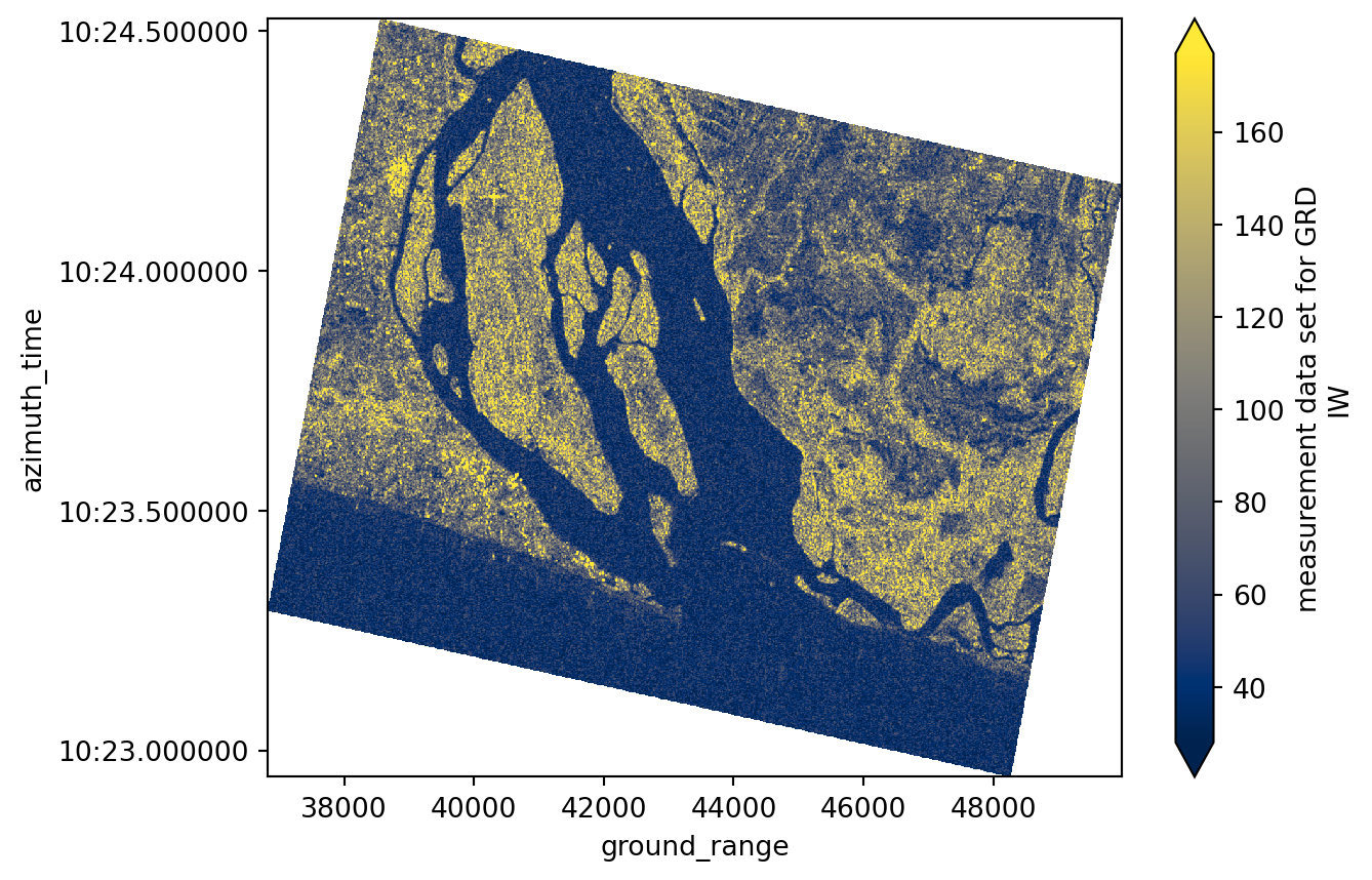
Radiometric calibration
In order to get a meanigful physical properties of features in the SAR scene that could be used for quantitative analysis, we need to apply a radiometric calibration on the backscatter values. This step converts the backscatter into a calibrated normalized radar cross section, correcting for incidence angle and sensor characteristics ensuring SAR images from different dates or viewing geometries are directly comparable.
- Reference: https://step.esa.int/docs/tutorials/S1TBX%20SAR%20Basics%20Tutorial.pdf
The radiometric calibration is done using the radiometric_calibration() function which takes the following keyword arguments:
grd:The GRD data array to be calibrated.calibration_ds: The calibration dataset containing the radiometric calibration lookup tables provided with the product. This dataset is interpolated to the GRD grid before being applied.calibration_type: The name of the calibration parameter to use from the calibration dataset. In this case,sigma_noughtis used to compute the sigma nought backscatter coefficient.
To have a look into the available data vars within the calibration dataset that could be used for the radiometric calibration
calibration.data_varsData variables:
beta_nought (azimuth_time, ground_range) float32 68kB dask.array<chunksize=(27, 632), meta=np.ndarray>
dn (azimuth_time, ground_range) float32 68kB dask.array<chunksize=(27, 632), meta=np.ndarray>
gamma (azimuth_time, ground_range) float32 68kB dask.array<chunksize=(27, 632), meta=np.ndarray>
sigma_nought (azimuth_time, ground_range) float32 68kB dask.array<chunksize=(27, 632), meta=np.ndarray>We apply the calibration, obtaining:
sigma_0 = radiometric_calibration(
grd=grd_subset, calibration_ds=calibration, calibration_type="sigma_nought"
)sigma_0<xarray.DataArray (azimuth_time: 1061, ground_range: 1316)> Size: 6MB
dask.array<pow, shape=(1061, 1316), dtype=float32, chunksize=(1061, 1316), chunktype=numpy.ndarray>
Coordinates:
* azimuth_time (azimuth_time) datetime64[ns] 8kB 2024-12-28T18:10:22.94533...
* ground_range (ground_range) float64 11kB 3.683e+04 3.684e+04 ... 4.998e+04
latitude (azimuth_time, ground_range) float64 11MB 5.739 ... 5.859
longitude (azimuth_time, ground_range) float64 11MB 0.6134 ... 0.7102sigma_0.plot(robust=True, cmap="cividis", cbar_kwargs={"label": "Sigma Nought"})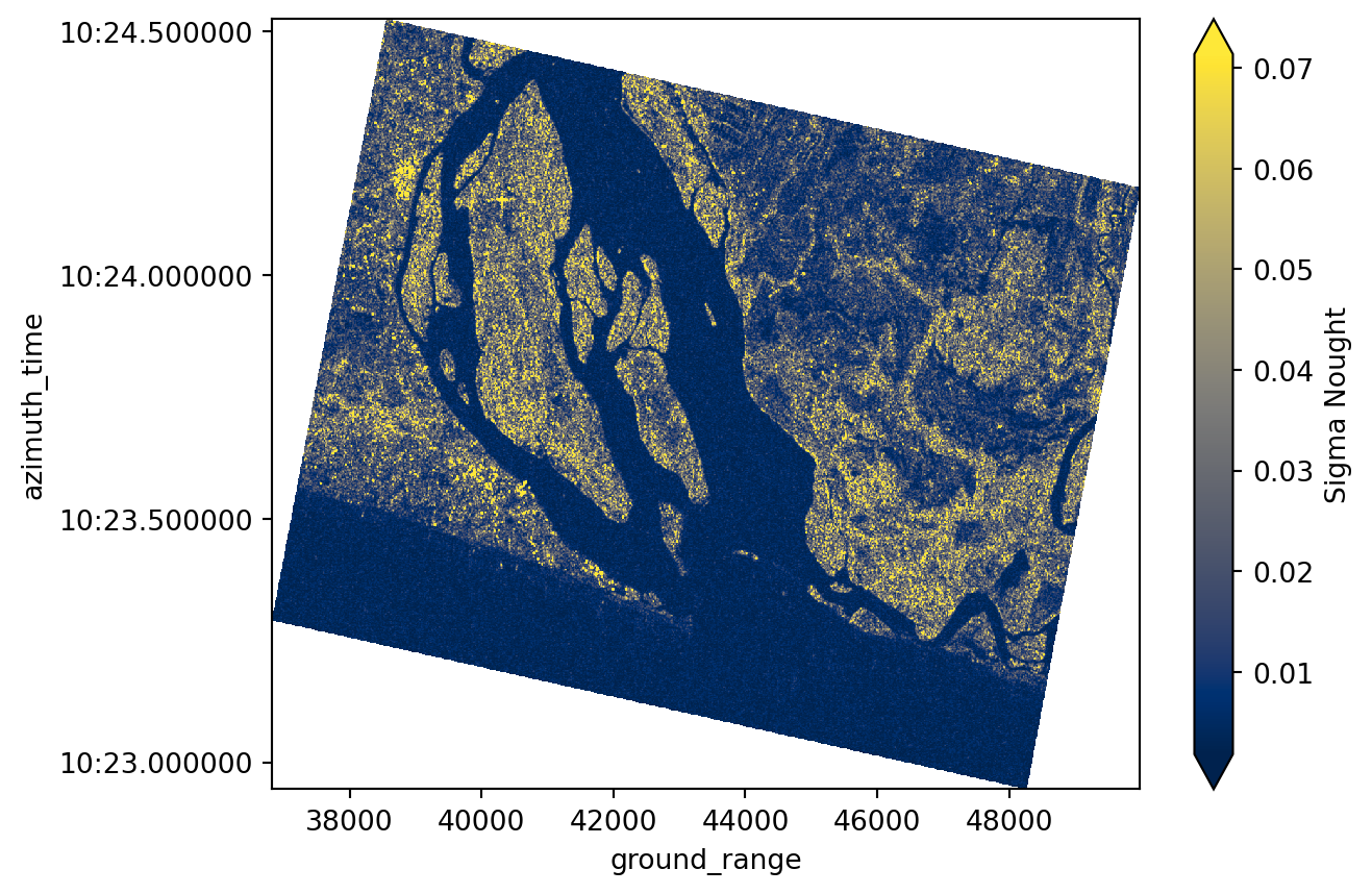
Speckel filtering
Raw SAR imagery is characterized by “grainy” or “salt and pepper” effect caused by random constructive and destructive interference, known as speckle. In order to reduce this effect and noise, we apply the spatial Lee Filter (Lee et al., 2009) that averages the pixel values while preserving edges.
For speckel filtering we will use the lee_filter_dask() function which takes the following keyword arguments:
da: The inputxarray.DataArrayto be filtered. Here,sigma_0is the radiometrically calibrated GRD subset.size: The size of the square moving window used to compute the local statistics for the Lee filter. Odd numbers are recommended (e.g., 5×5). Larger windows produce stronger smoothing but may reduce spatial detail.
sigma_0_spk = lee_filter_dask(da=sigma_0, size=5)sigma_0_spk<xarray.DataArray (azimuth_time: 1061, ground_range: 1316)> Size: 6MB
dask.array<transpose, shape=(1061, 1316), dtype=float32, chunksize=(1061, 1316), chunktype=numpy.ndarray>
Coordinates:
* azimuth_time (azimuth_time) datetime64[ns] 8kB 2024-12-28T18:10:22.94533...
* ground_range (ground_range) float64 11kB 3.683e+04 3.684e+04 ... 4.998e+04
latitude (azimuth_time, ground_range) float64 11MB 5.739 ... 5.859
longitude (azimuth_time, ground_range) float64 11MB 0.6134 ... 0.7102
Attributes:
attrs: {'speckle filter method': 'lee'}Obtaining a cleaner image
sigma_0_spk.plot(robust=True, cmap="cividis", cbar_kwargs={"label": "Sigma Nought"})
plt.title("Sigma Nought after Lee Filter")
plt.show()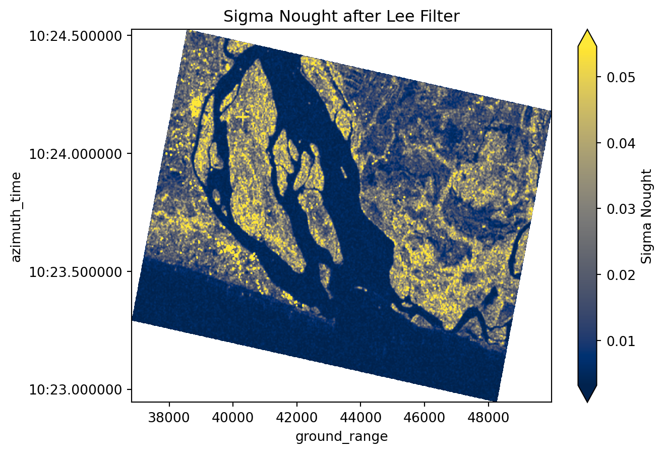
Georefrecing and regredding
Sentinel-1 GRD Zarr comes in irregular image geometry that does not align with common geographic grids. In order to conduct spatial analysis, and scenes comparison, and mapping, we need to georefrence and resample the data onto a regular grid.
We will use an ODC GeoBox along with with scipy.griddata to interpolate the SAR values onto a consistent latitude-longitude grid. These utilities are available within the regrid() function which takes the following keyword arguments:
da: The inputxarray.DataArrayto regrid. Here,sigma_0_spkis the speckle-filtered GRD subset.bounds: The geographic bounding box for the output grid:[min_lon, min_lat, max_lon, max_lat].resolution: Tuple(dx, dy)defining the grid spacing in the coordinate units of the CRS. For example,10 / 111320degrees corresponds roughly to 10 meters.crs: Coordinate reference system of the output grid (default is"EPSG:4326"for WGS84).method: Interpolation method for mapping irregularly spaced data to the regular grid. Options include"nearest","linear", or"cubic".
resolution = 10 / 111320 # approx 10 meters in degrees
crs = "epsg:4326"
sigma_0_spk_geo = regrid(
da=sigma_0_spk,
bounds=aoi_bounds,
resolution=resolution,
crs=crs,
method="nearest", # "linear" or "cubic"
)sigma_0_spk_geo<xarray.DataArray (y: 868, x: 1175)> Size: 8MB
array([[0.02022304, 0.02022304, 0.0271727 , ..., 0.00480022, 0.00438391,
0.00438391],
[0.02022304, 0.02022304, 0.0271727 , ..., 0.00480022, 0.0070433 ,
0.0070433 ],
[0.02168461, 0.02168461, 0.02967146, ..., 0.00716109, 0.00948818,
0.00948818],
...,
[0.00227514, 0.00227514, 0.00214053, ..., 0.00365857, 0.00334549,
0.00260707],
[0.00176132, 0.00176132, 0.00177638, ..., 0.00396993, 0.00376833,
0.00376833],
[0.00176132, 0.00177638, 0.00177638, ..., 0.00396993, 0.00376833,
0.00376833]], shape=(868, 1175))
Coordinates:
* y (y) float64 7kB 5.838 5.838 5.838 5.837 ... 5.76 5.76 5.76 5.76
* x (x) float64 9kB 0.6091 0.6092 0.6093 ... 0.7144 0.7145 0.7146
spatial_ref int64 8B 0
Attributes:
interpolation: nearest
odcgeobox: GeoBox((868, 1175), Affine(8.983111749910169e-05, 0.0, 0....sigma_0_spk_geo.odcgeoboxGeoBox
Dimensions
1,175x868
EPSG
4326
Resolution
8.98311e-05°
Cell
200px
WKT
GEOGCRS["WGS 84",
ENSEMBLE["World Geodetic System 1984 ensemble",
MEMBER["World Geodetic System 1984 (Transit)"],
MEMBER["World Geodetic System 1984 (G730)"],
MEMBER["World Geodetic System 1984 (G873)"],
MEMBER["World Geodetic System 1984 (G1150)"],
MEMBER["World Geodetic System 1984 (G1674)"],
MEMBER["World Geodetic System 1984 (G1762)"],
MEMBER["World Geodetic System 1984 (G2139)"],
MEMBER["World Geodetic System 1984 (G2296)"],
ELLIPSOID["WGS 84",6378137,298.257223563,
LENGTHUNIT["metre",1]],
ENSEMBLEACCURACY[2.0]],
PRIMEM["Greenwich",0,
ANGLEUNIT["degree",0.0174532925199433]],
CS[ellipsoidal,2],
AXIS["geodetic latitude (Lat)",north,
ORDER[1],
ANGLEUNIT["degree",0.0174532925199433]],
AXIS["geodetic longitude (Lon)",east,
ORDER[2],
ANGLEUNIT["degree",0.0174532925199433]],
USAGE[
SCOPE["Horizontal component of 3D system."],
AREA["World."],
BBOX[-90,-180,90,180]],
ID["EPSG",4326]]
sigma_0_spk_geo.plot(robust=True, cmap="cividis", cbar_kwargs={"label": "Sigma Nought"})
plt.title("Regridded Sigma Nought after Lee Filter")
plt.show()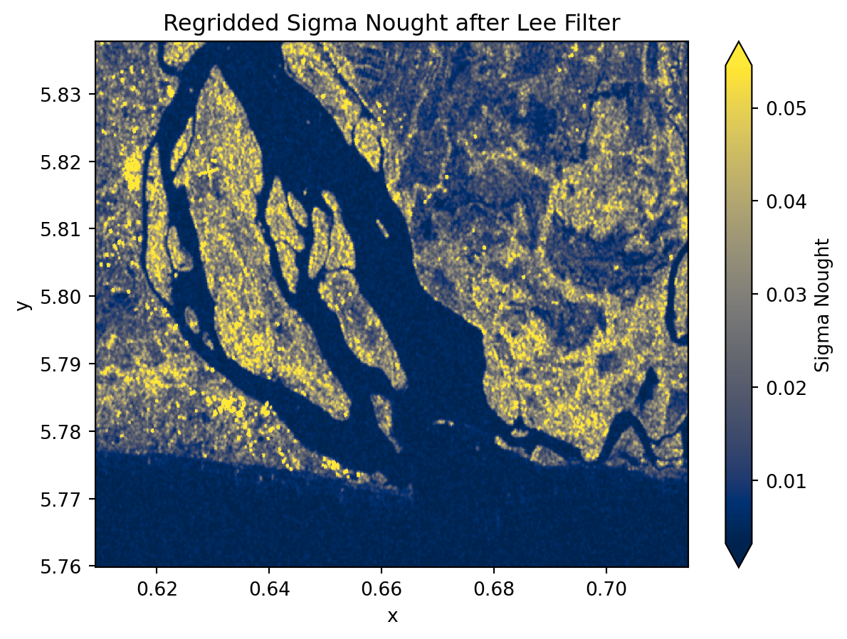
Convert backscatter to dB
We convert the regridded sigma_0 backscatter intensity from Linear scale to decibels (dB) using a logarithmic transformation. This enhances contrast and simplifies statistical analysis and interpretation of the image. It is considered a standard approach for representing SAR intensity.
sigma_0_spk_geo_db = 10 * np.log10(sigma_0_spk_geo)sigma_0_spk_geo_db<xarray.DataArray (y: 868, x: 1175)> Size: 8MB
array([[-16.94153556, -16.94153556, -15.65867213, ..., -23.18738561,
-23.58138141, -23.58138141],
[-16.94153556, -16.94153556, -15.65867213, ..., -23.18738561,
-21.52223657, -21.52223657],
[-16.63848472, -16.63848472, -15.27661105, ..., -21.45021141,
-20.22816859, -20.22816859],
...,
[-26.42991425, -26.42991425, -26.69479123, ..., -24.36688424,
-24.75540359, -25.8384678 ],
[-27.54160746, -27.54160746, -27.50464296, ..., -24.01217139,
-24.2385137 , -24.2385137 ],
[-27.54160746, -27.50464296, -27.50464296, ..., -24.01217139,
-24.2385137 , -24.2385137 ]], shape=(868, 1175))
Coordinates:
* y (y) float64 7kB 5.838 5.838 5.838 5.837 ... 5.76 5.76 5.76 5.76
* x (x) float64 9kB 0.6091 0.6092 0.6093 ... 0.7144 0.7145 0.7146
spatial_ref int64 8B 0
Attributes:
interpolation: nearest
odcgeobox: GeoBox((868, 1175), Affine(8.983111749910169e-05, 0.0, 0....sigma_0_spk_geo_db.plot(
robust=True, cmap="cividis", cbar_kwargs={"label": "Sigma Nought dB"}
)
plt.title("Calibrated Sigma Nought in dB")
plt.show()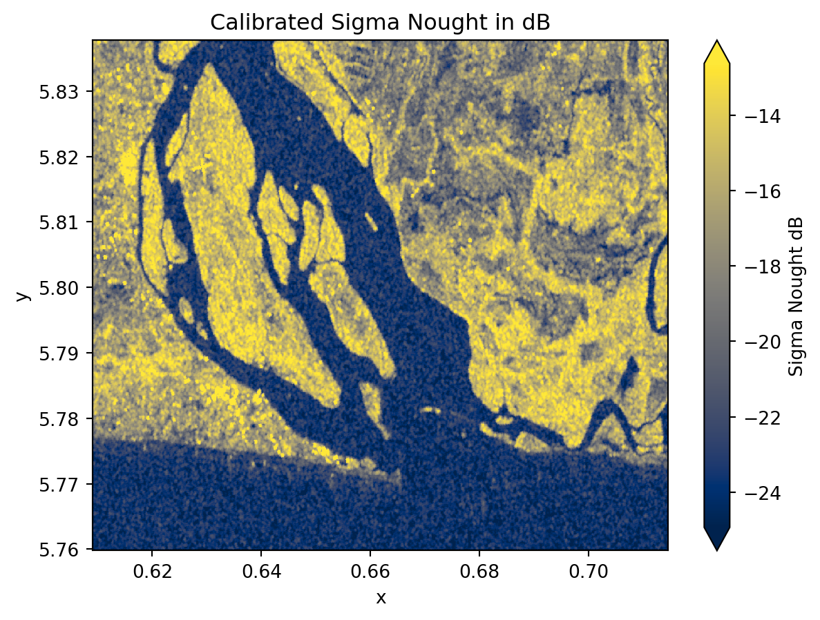
sigma_0_spk_geo_db.hvplot.image(
x="x",
y="y",
robust=True,
cmap="cividis",
title="SAR GRD",
)Water mask
To separate water from non-water surfaces, we first inspect the distribution of backscatter values using a histogram. In the following histogram we could choose -19 as therhold.
plt.hist(sigma_0_spk_geo_db.values.ravel(), bins=50, alpha=0.7)
plt.title("Histogram of Sigma Nought (dB) Values")
plt.show()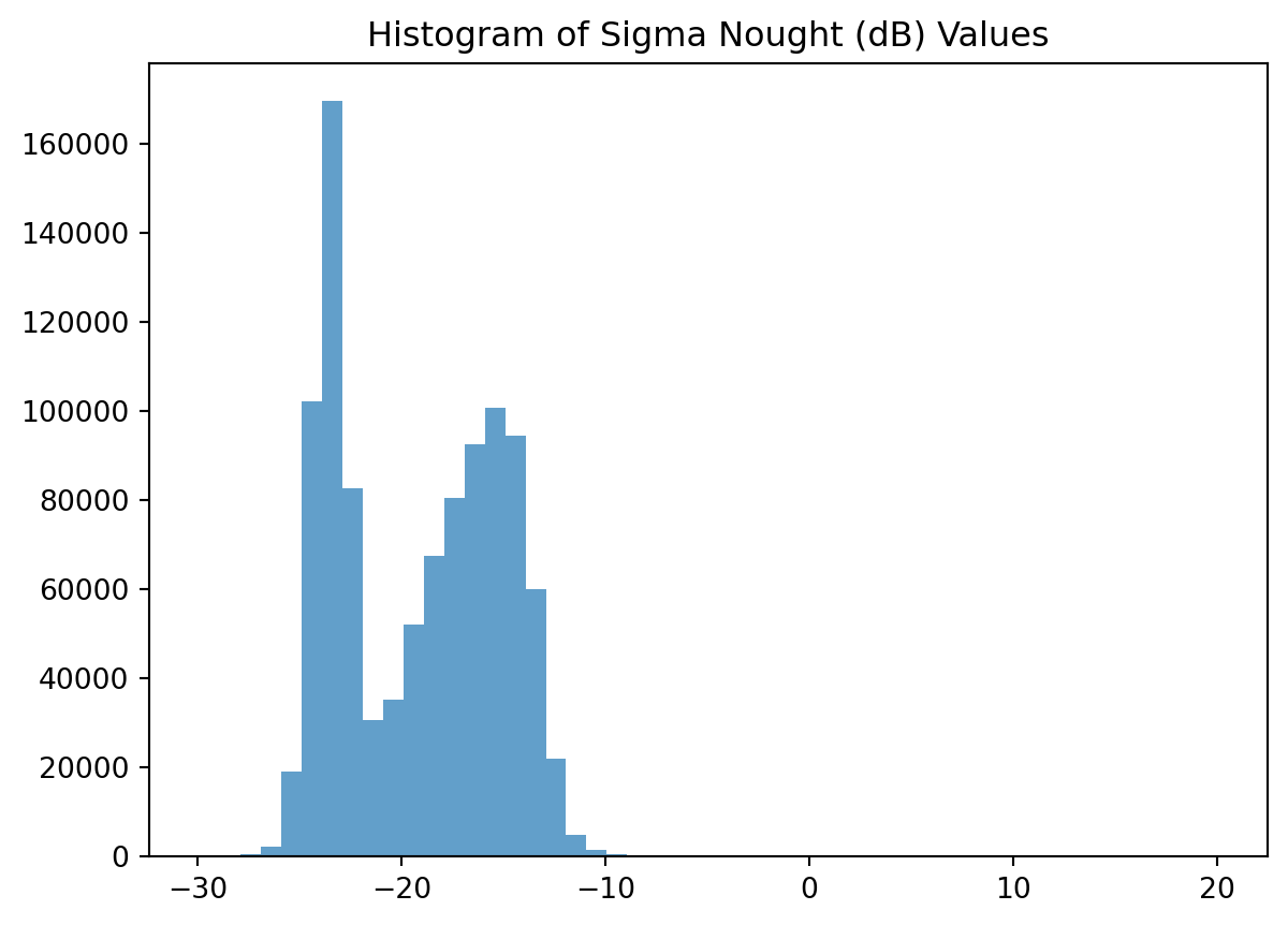
Since SAR water thresholds vary across scenes and times, a fixed cutoff is unreliable. Threfore, we apply an adaptative thresholding method using Otsu algorithm provided by skimage, which automatically determines an optimal threshold from the intensity distribution and create a water mask accordingly. This algorithm is available within xr_threshold_otsu function which takes the following keyword arguments:
da: Inputxarray.DataArrayto threshold.mask_nan: If True (default), any NaN values are ignored during threshold computation.return_threshold: If True, the calculated threshold value is stored as an attribute of the resulting mask.mask_name: Optional name for the binary mask DataArray. This helps with metadata or when saving to file.
water_mask = xr_threshold_otsu(
da=sigma_0_spk_geo_db, mask_nan=True, return_threshold=True, mask_name="water_mask"
)
print(f"Otsu threshold: {water_mask.attrs['threshold']}")Otsu threshold: -19.460939955179214water_mask<xarray.DataArray 'water_mask' (y: 868, x: 1175)> Size: 1MB
array([[1, 1, 1, ..., 0, 0, 0],
[1, 1, 1, ..., 0, 0, 0],
[1, 1, 1, ..., 0, 0, 0],
...,
[0, 0, 0, ..., 0, 0, 0],
[0, 0, 0, ..., 0, 0, 0],
[0, 0, 0, ..., 0, 0, 0]], shape=(868, 1175), dtype=uint8)
Coordinates:
* y (y) float64 7kB 5.838 5.838 5.838 5.837 ... 5.76 5.76 5.76 5.76
* x (x) float64 9kB 0.6091 0.6092 0.6093 ... 0.7144 0.7145 0.7146
spatial_ref int64 8B 0
Attributes:
threshold: -19.460939955179214(1 - water_mask).plot(cmap="Blues")
plt.title("Water Mask (1 = Water, 0 = Non-Water)")
plt.show()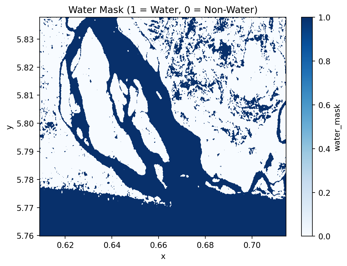
(1 - water_mask).hvplot.image(
x="x",
y="y",
cmap="Blues",
robust=True,
title="Water Mask",
)Time series analysis
So far we have walked through each processing step separately. To automate the workflow and apply it efficiently across Sentinel-1 acquisitions, we could now wrap all these operations into a single processing function process_item. This allows us to automatically generate water masks for every item in our STAC collection.
def process_item(
item, aoi_bounds, polarization="VH", resolution=10 / 111320, crs="epsg:4326"
):
"""Process a STAC item to generate water mask and timestamp."""
url = item.assets["product"].href
store = fsspec.get_mapper(url)
datatree = xr.open_datatree(store, engine="zarr", chunks={})
group_VH = [x for x in datatree.children if f"{polarization}" in x][0]
grd = datatree[group_VH]["measurements/grd"]
gcp = datatree[group_VH]["conditions/gcp"].to_dataset()
calibration = datatree[group_VH]["quality/calibration"].to_dataset()
grd_subset = subset(grd, gcp, aoi_bounds, offset=1)
sigma_0 = radiometric_calibration(
grd_subset, calibration, calibration_type="sigma_nought"
)
sigma_0_spk = lee_filter_dask(sigma_0, size=5)
sigma_0_spk_geo = regrid(
da=sigma_0_spk,
bounds=aoi_bounds,
resolution=resolution,
crs=crs,
method="nearest",
)
sigma_0_spk_geo_db = 10 * np.log10(sigma_0_spk_geo)
water_mask = xr_threshold_otsu(
sigma_0_spk_geo_db, return_threshold=True, mask_name="water_mask"
)
t = np.datetime64(item.properties["datetime"][:-2], "ns")
water_mask = water_mask.assign_coords(time=t)
return water_maskNow we loop through all STAC items and use the process_item to build the full water-mask dataset.
water_masks = []
thresholds = []
for item in tqdm(items):
water_mask = process_item(item, aoi_bounds)
water_masks.append(1 - water_mask) # invert mask to have 1 = water
thresholds.append(water_mask.attrs["threshold"])
water_mask_ds = xr.concat(water_masks, dim="time")
water_mask_ds = water_mask_ds.assign_coords(threshold=("time", thresholds)).sortby(
"time"
)water_mask_ds<xarray.DataArray 'water_mask' (time: 30, y: 868, x: 1175)> Size: 31MB
array([[[0, 0, 0, ..., 1, 0, 0],
[0, 0, 0, ..., 0, 0, 0],
[0, 0, 0, ..., 0, 0, 0],
...,
[1, 1, 1, ..., 1, 1, 1],
[1, 1, 1, ..., 1, 1, 1],
[1, 1, 1, ..., 1, 1, 1]],
[[0, 0, 0, ..., 1, 0, 0],
[0, 0, 0, ..., 0, 0, 0],
[0, 0, 0, ..., 0, 0, 0],
...,
[1, 1, 1, ..., 1, 1, 1],
[1, 1, 1, ..., 1, 1, 1],
[1, 1, 1, ..., 1, 1, 1]],
[[0, 0, 0, ..., 0, 0, 0],
[0, 0, 0, ..., 0, 0, 0],
[0, 0, 0, ..., 0, 0, 0],
...,
...
...,
[1, 1, 1, ..., 1, 1, 1],
[1, 1, 1, ..., 1, 1, 1],
[1, 1, 1, ..., 1, 1, 1]],
[[0, 0, 0, ..., 0, 0, 0],
[0, 0, 0, ..., 0, 0, 0],
[0, 0, 0, ..., 0, 0, 0],
...,
[1, 1, 1, ..., 1, 1, 1],
[1, 1, 1, ..., 1, 1, 1],
[1, 1, 1, ..., 1, 1, 1]],
[[0, 0, 0, ..., 1, 1, 1],
[0, 0, 0, ..., 1, 1, 1],
[0, 0, 0, ..., 1, 1, 1],
...,
[1, 1, 1, ..., 1, 1, 1],
[1, 1, 1, ..., 1, 1, 1],
[1, 1, 1, ..., 1, 1, 1]]], shape=(30, 868, 1175), dtype=uint8)
Coordinates:
* time (time) datetime64[ns] 240B 2024-01-03T18:10:33.162880 ... 20...
threshold (time) float64 240B -19.52 -19.6 -19.52 ... -19.53 -19.46
* y (y) float64 7kB 5.838 5.838 5.838 5.837 ... 5.76 5.76 5.76 5.76
* x (x) float64 9kB 0.6091 0.6092 0.6093 ... 0.7144 0.7145 0.7146
spatial_ref int64 8B 0
Attributes:
threshold: -19.460939955179214# Check the water mask thresholds over time
plt.plot(water_mask_ds.time, water_mask_ds.threshold, marker="o")
plt.title("Water Mask Thresholds over Time")
plt.show()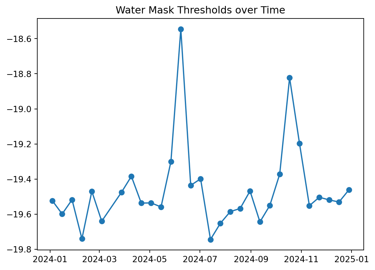
dates = water_mask_ds.time
dates<xarray.DataArray 'time' (time: 30)> Size: 240B
array(['2024-01-03T18:10:33.162880000', '2024-01-15T18:10:32.384560000',
'2024-01-27T18:10:32.348240000', '2024-02-08T18:10:31.840520000',
'2024-02-20T18:10:31.704330000', '2024-03-03T18:10:32.017430000',
'2024-03-27T18:10:32.063920000', '2024-04-08T18:10:32.818500000',
'2024-04-20T18:10:33.125570000', '2024-05-02T18:10:33.422470000',
'2024-05-14T18:10:32.697480000', '2024-05-26T18:10:33.280330000',
'2024-06-07T18:10:32.518290000', '2024-06-19T18:10:32.151680000',
'2024-07-01T18:10:31.407790000', '2024-07-13T18:10:31.135470000',
'2024-07-25T18:10:30.555910000', '2024-08-06T18:10:30.686650000',
'2024-08-18T18:10:30.998140000', '2024-08-30T18:10:30.942770000',
'2024-09-11T18:10:31.320170000', '2024-09-23T18:10:31.807580000',
'2024-10-05T18:10:32.220710000', '2024-10-17T18:10:32.467090000',
'2024-10-29T18:10:32.354540000', '2024-11-10T18:10:31.932980000',
'2024-11-22T18:10:31.006880000', '2024-12-04T18:10:30.239490000',
'2024-12-16T18:10:29.146030000', '2024-12-28T18:10:30.445130000'],
dtype='datetime64[ns]')
Coordinates:
* time (time) datetime64[ns] 240B 2024-01-03T18:10:33.162880 ... 20...
threshold (time) float64 240B -19.52 -19.6 -19.52 ... -19.53 -19.46
spatial_ref int64 8B 0Lets inspect the water mask for the first 4 dates.
water_mask_ds.sel(time=dates[:4]).plot(col="time", cmap="Blues", vmin=0, vmax=1)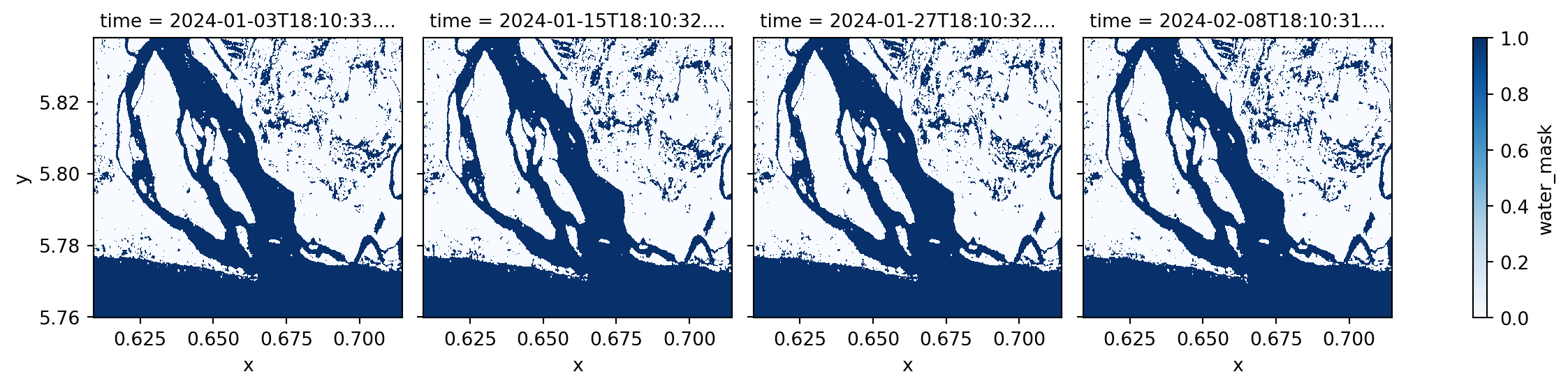
We found out that the RAW Sentinel-1 GRD scene for 2024-06-07 has issues and artificat that will lead to incorrect water classification. Therefore, we will exclude it from our water frequency analysis.
bad_date = pd.to_datetime("2024-06-07").date()
filtered_water_ds = water_mask_ds.sel(
time=water_mask_ds.time.to_index().date != bad_date
)filtered_water_ds<xarray.DataArray 'water_mask' (time: 29, y: 868, x: 1175)> Size: 30MB
array([[[0, 0, 0, ..., 1, 0, 0],
[0, 0, 0, ..., 0, 0, 0],
[0, 0, 0, ..., 0, 0, 0],
...,
[1, 1, 1, ..., 1, 1, 1],
[1, 1, 1, ..., 1, 1, 1],
[1, 1, 1, ..., 1, 1, 1]],
[[0, 0, 0, ..., 1, 0, 0],
[0, 0, 0, ..., 0, 0, 0],
[0, 0, 0, ..., 0, 0, 0],
...,
[1, 1, 1, ..., 1, 1, 1],
[1, 1, 1, ..., 1, 1, 1],
[1, 1, 1, ..., 1, 1, 1]],
[[0, 0, 0, ..., 0, 0, 0],
[0, 0, 0, ..., 0, 0, 0],
[0, 0, 0, ..., 0, 0, 0],
...,
...
...,
[1, 1, 1, ..., 1, 1, 1],
[1, 1, 1, ..., 1, 1, 1],
[1, 1, 1, ..., 1, 1, 1]],
[[0, 0, 0, ..., 0, 0, 0],
[0, 0, 0, ..., 0, 0, 0],
[0, 0, 0, ..., 0, 0, 0],
...,
[1, 1, 1, ..., 1, 1, 1],
[1, 1, 1, ..., 1, 1, 1],
[1, 1, 1, ..., 1, 1, 1]],
[[0, 0, 0, ..., 1, 1, 1],
[0, 0, 0, ..., 1, 1, 1],
[0, 0, 0, ..., 1, 1, 1],
...,
[1, 1, 1, ..., 1, 1, 1],
[1, 1, 1, ..., 1, 1, 1],
[1, 1, 1, ..., 1, 1, 1]]], shape=(29, 868, 1175), dtype=uint8)
Coordinates:
* time (time) datetime64[ns] 232B 2024-01-03T18:10:33.162880 ... 20...
threshold (time) float64 232B -19.52 -19.6 -19.52 ... -19.53 -19.46
* y (y) float64 7kB 5.838 5.838 5.838 5.837 ... 5.76 5.76 5.76 5.76
* x (x) float64 9kB 0.6091 0.6092 0.6093 ... 0.7144 0.7145 0.7146
spatial_ref int64 8B 0
Attributes:
threshold: -19.460939955179214Monthly surface water frequency
Now that we have the water masks, we can group them by month, compute the average water presence for each pixel, and convert it to a percentage (%) to represent monthly water frequency.
monthly_water_frequency = filtered_water_ds.groupby("time.month").mean("time") * 100
monthly_water_frequency.name = "SWF"
month_names = pd.date_range(start="2024-01-01", periods=12, freq="ME").strftime("%B")
monthly_water_frequency.coords["month"] = ("month", month_names)
monthly_water_frequency = monthly_water_frequency.assign_attrs(
long_name="Surface Water Frequency"
)
monthly_water_frequency = monthly_water_frequency.assign_attrs(units="%")
monthly_water_frequency<xarray.DataArray 'SWF' (month: 12, y: 868, x: 1175)> Size: 98MB
array([[[ 0. , 0. , 0. , ..., 66.66666667,
0. , 0. ],
[ 0. , 0. , 0. , ..., 0. ,
0. , 0. ],
[ 0. , 0. , 0. , ..., 0. ,
0. , 0. ],
...,
[100. , 100. , 100. , ..., 100. ,
100. , 100. ],
[100. , 100. , 100. , ..., 100. ,
100. , 100. ],
[100. , 100. , 100. , ..., 100. ,
100. , 100. ]],
[[ 0. , 0. , 0. , ..., 50. ,
50. , 0. ],
[ 0. , 0. , 0. , ..., 50. ,
0. , 0. ],
[ 50. , 0. , 0. , ..., 0. ,
0. , 0. ],
...
[100. , 100. , 100. , ..., 100. ,
100. , 100. ],
[100. , 100. , 100. , ..., 100. ,
100. , 100. ],
[100. , 100. , 100. , ..., 100. ,
100. , 100. ]],
[[ 0. , 0. , 0. , ..., 66.66666667,
33.33333333, 33.33333333],
[ 0. , 0. , 0. , ..., 33.33333333,
33.33333333, 33.33333333],
[ 0. , 0. , 0. , ..., 33.33333333,
33.33333333, 33.33333333],
...,
[100. , 100. , 100. , ..., 100. ,
100. , 100. ],
[100. , 100. , 100. , ..., 100. ,
100. , 100. ],
[100. , 100. , 100. , ..., 100. ,
100. , 100. ]]], shape=(12, 868, 1175))
Coordinates:
* month (month) object 96B 'January' 'February' ... 'December'
* y (y) float64 7kB 5.838 5.838 5.838 5.837 ... 5.76 5.76 5.76 5.76
* x (x) float64 9kB 0.6091 0.6092 0.6093 ... 0.7144 0.7145 0.7146
spatial_ref int64 8B 0
Attributes:
threshold: -19.460939955179214
long_name: Surface Water Frequency
units: %monthly_water_frequency.plot(col="month", col_wrap=4, cmap="Blues", robust=True)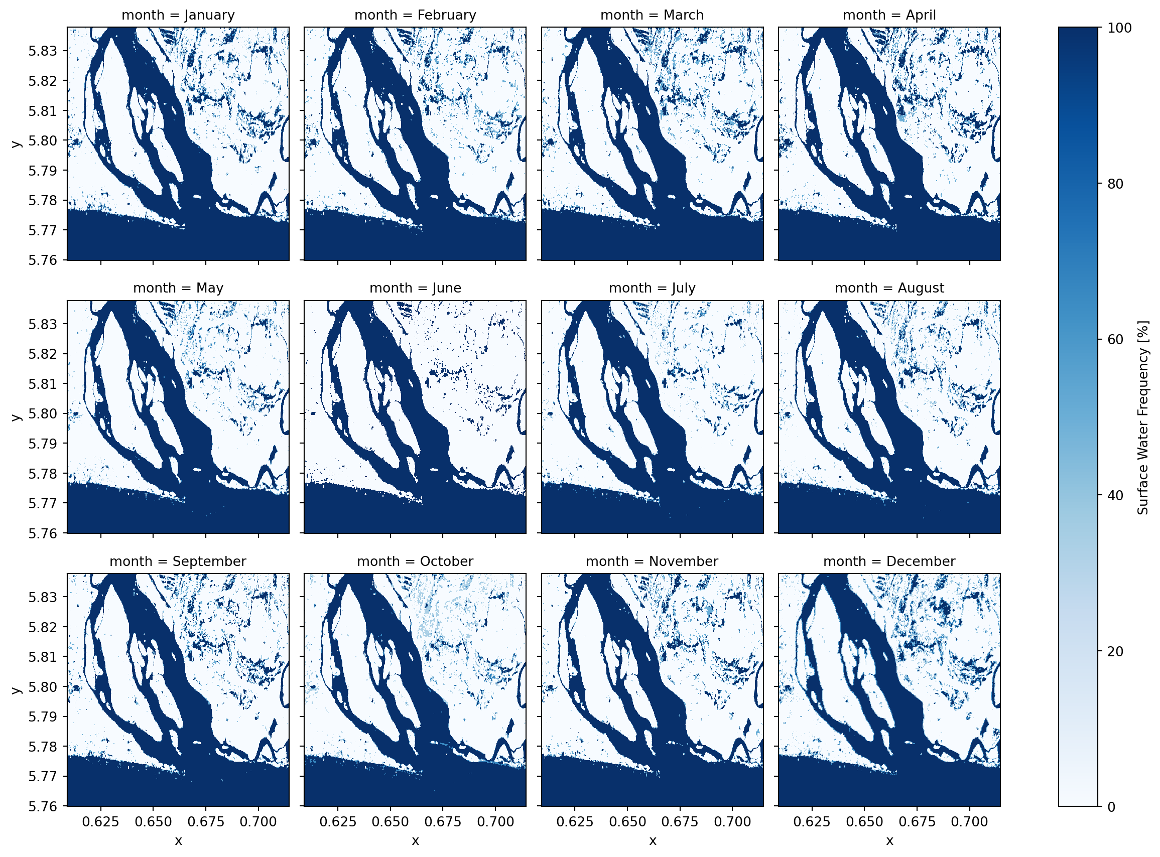
Annual surface water frequency
Lets calculates the average water occurence across the entire time series over the year.
annual_water_frequency = filtered_water_ds.mean("time") * 100
annual_water_frequency = annual_water_frequency.assign_attrs(
long_name="Surface Water Frequency"
)
annual_water_frequency = annual_water_frequency.assign_attrs(units="%")annual_water_frequency.plot(cmap="Blues")
plt.title("Annual Surface Water Frequency (%)")
plt.show()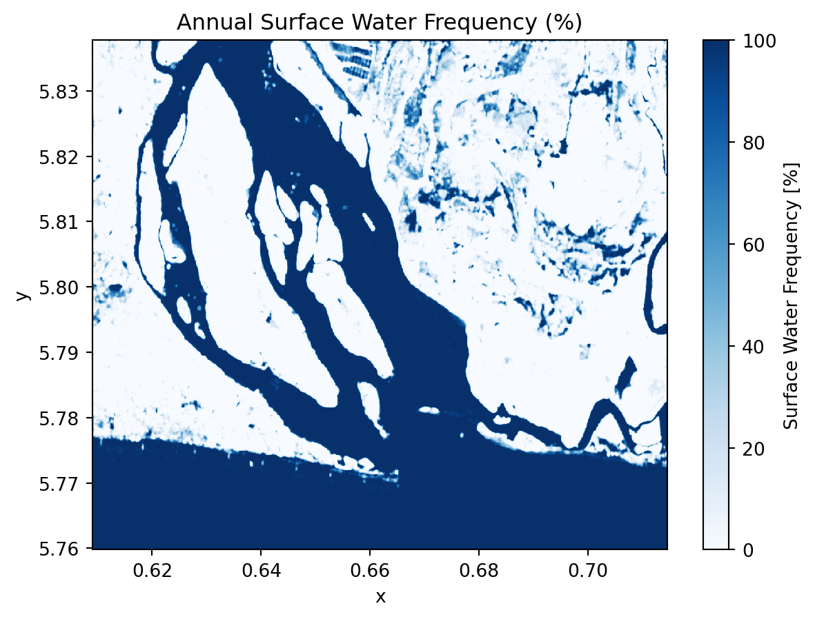
annual_water_frequency.hvplot.image(
x="x",
y="y",
robust=True,
cmap="Blues",
title="Annual Surface Water Frequency (%)",
)Annual water change
We could also computes the standard deviation of water presence over time. This highlights areas with high water variability (seasonal or dynamic water bodies).
annual_water_change = filtered_water_ds.std("time") * 100
annual_water_change = annual_water_change.assign_attrs(
long_name="Surface Water Variation"
)
annual_water_change = annual_water_change.assign_attrs(units="%")annual_water_change.plot(cmap="magma")
plt.title("Annual Surface Water Variation")
plt.show()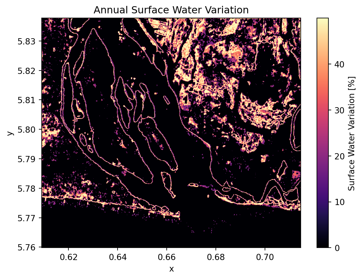
annual_water_change.hvplot.image(
x="x",
y="y",
robust=True,
cmap="magma",
title="Annual Surface Water Variation",
)💪 Now it is your turn
congratulations 🎉
We have worked through the complete workflow for analyzing Sentinel-1 surface water dynamics from .zarr data. Now it is your turn to explore and expand the analysis in the following ways:
Task 1: Explore your own area of interest
Choose a different wetland, lake system, river delta, or floodplain anywhere in the world. Use different STAC search configurations (aoi_bounds, date_start, date_end) and derive the:
- Seasonal variation
- Maximum water extent
- Minumum water extent
- Long-term changes in water extent (more than 1 year of data)
Task 2: Experiment with other polarizations and combinations
Instead of relying solely on VH for water extraction try:
VVpolarizationVH/VVratio- Dual-polarization thresholding or machine learning classification (Kreiser, Z. et al., 2018)
Task 3: Compare or integrate Sentinel-1 with Sentinel-2
Design a workflow for Sentinel-2 water detection and consider using spectral indices such as the Normalized Difference Water Index (NDWI) Gao, 1996 or the Modified Normalized Difference Water Index (mNDWI) Xu, 2006.
Compare Sentinel-2 water dectection with our Sentinel-1 workflow.
Recent studies show that combining Sentinel-1 and Sentinel-2 data can improve water detection (Bioresita et al., 2019; Kaplan and Avdan 2018). Consider exploring methods that fuse the information from both sensors.
Conclusion
In this notebook, we demonstrated how to use Sentinel-1 data in .zarr format for time-series analysis of surface water dynamics in a wetland coastal and cloudy-prone area. The zarr structure is especially useful for efficient extraction of data over a specific area of interest without loading the full dataset.
We developed a streamlined time series workflow using pystac-client and the EODC STAC API to preprocess Sentinel-1 GRD data. This included spatial subsetting, radiometric calibration, speckle filtering, georeferencing, and regridding. We also implemented an automated process for surface water detection and derived surface water occurrence, frequency, and change.
Note: Although in this notebook we opted to use VH polarization to detect the water, users may also experiment with VV polarization or combine both polarizations for improved water detection, and implement their own methods for deriving surface water masks. This workflow can also be adapted for other applications, such as monitoring lake dynamic and flood events.
What’s next?
In the following notebook, we will explore the integration of a Sentinel-2 and Sentinel-3 time series using a highly efficient and scalable fusion method - EFAST.