Flood Mapping - Time Series Analysis in Valencia

Introduction

Sentinel-1 GRD data is particularly valuable to detect water and underwater areas. Synthetic Aperture Radar (SAR) can capture images day and night, in any weather, a feature especially important for flooding events, where cloudy and rainy weather can persist for weeks. This makes it far more reliable than optical sensors during storms.

With its frequent revisits, wide coverage, and free high-resolution data, Sentinel-1 enables the rapid mapping of flood extents, as will be demonstrated in this workflow. VV polarization is preferred for flood mapping due to its sensitivity to water surfaces, which typically appear darker in the images compared to land surfaces.

The Flooding Event

On October 29, 2024, the city of Valencia (Spain) was hit by catastrophic flooding caused by intense storms, leaving over 230 deaths and billions in damages. This disaster was part of Europe’s worst flood year in over a decade, with hundreds of thousands affected continent-wide. Such events highlight the urgent need for reliable flood monitoring to support emergency response, damage assessment and long-term resilience planning.

With respect to this event, we will demonstrate how to use Sentinel-1 GRD data to map flood extents. We will use 14 Sentinel-1 GRD images from the IW swath, covering the city and metropolitan area of Valencia from October 7, 2024 to March 24, 2025. This includes 2 images captured before, 1 immediately after the heavy rains, and 11 images taken after the flooding event, until the water levels got back to normal: - October 7, 2424 (before) - October 19, 2024 (before) - October 31, 2024 (right after the event) - November 12, 2024 (after) - November 24, 2024 (after) - December 6, 2024 (after) - December 18, 2024 (after) - December 30, 2024 (after) - January 11, 2025 (after) - January 23, 2025 (after) - February 4, 2025 (after) - February 16, 2025 (after) - March 12, 2025 (after) - March 24, 2025 (after)

What we will learn

🌊 How to create a workflow to map flood events.
⚒️ Basic SAR processing tools.
📊 How to create a data cube to perform time series analysis.

Import libraries

import xarray as xr 
# import xarray_sentinel 
import pandas as pd
import matplotlib as plt
import matplotlib.pyplot as plt
import numpy as np
from scipy.interpolate import griddata

import dask                             # these last two libraries are imported to open the datasets faster
from dask.distributed import Client     # and in the end take advantage of the optimized .zarr format

Data pre-processing

To search and load the data needed for the analysis, we will follow the processes we presented in Sentinel-1 GRD structure tutorial and S1 basic operations tutorial.

Once we defined our interest Sentinel-1 GRD items, we can see that they contain both VH and VV polarizations.
For this flood mapping context, VV polarization is the choice of interest, as water backscatter is much more visible with it, rather than with VH.

Loading the datatree

The list below shows the names of the products we will use for the flood mapping and time series analysis.
As we have seen in previous chapters, these names already contain valuable information that can be used to search for specific products within the EOPF STAC catalogue.

scenes = ["S1A_IW_GRDH_1SDV_20241007T180256_20241007T180321_056000_06D943_D46B", 
          "S1A_IW_GRDH_1SDV_20241019T180256_20241019T180321_056175_06E02E_2D52", 
          "S1A_IW_GRDH_1SDV_20241031T180256_20241031T180321_056350_06E71E_479F", 
          "S1A_IW_GRDH_1SDV_20241112T180255_20241112T180320_056525_06EE16_DC29", 
          "S1A_IW_GRDH_1SDV_20241124T180254_20241124T180319_056700_06F516_BA27", 
          "S1A_IW_GRDH_1SDV_20241206T180253_20241206T180318_056875_06FBFD_25AD", 
          "S1A_IW_GRDH_1SDV_20241218T180252_20241218T180317_057050_0702F2_0BC2", 
          "S1A_IW_GRDH_1SDV_20241230T180251_20241230T180316_057225_0709DD_15AC", 
          "S1A_IW_GRDH_1SDV_20250111T180250_20250111T180315_057400_0710C7_ADBB", 
          "S1A_IW_GRDH_1SDV_20250123T180249_20250123T180314_057575_0717B9_A784", 
          "S1A_IW_GRDH_1SDV_20250204T180249_20250204T180314_057750_071EA2_4373", 
          "S1A_IW_GRDH_1SDV_20250216T180248_20250216T180313_057925_0725AE_8AC7", 
          "S1A_IW_GRDH_1SDV_20250312T180248_20250312T180313_058275_0733E6_4F5B", 
          "S1A_IW_GRDH_1SDV_20250324T180248_20250324T180313_058450_073AD0_04B7", 
          ]

zarr_paths = []
for scene in scenes:
    zarr_paths.append(f"https://objects.eodc.eu/e05ab01a9d56408d82ac32d69a5aae2a:notebook-data/tutorial_data/cpm_v260/{scene}.zarr")

Next, we will load all zarr datasets as xarray.Datatrees. Here we are not reading the entire dataset from the store; but, creating a set of references to the data, which enables us to access it efficiently later in the analysis.

client = Client()  # Set up local cluster on your laptop
client

@dask.delayed
def load_datatree_delayed(path):
    return xr.open_datatree(path, engine="zarr", consolidated=True, chunks="auto")

# Create delayed objects
delayed_datatrees = [load_datatree_delayed(path) for path in zarr_paths]
# Compute in parallel
datatrees = dask.compute(*delayed_datatrees)

Each element inside the datatree list is a datatree and corresponds to a Sentinel-1 GRD scene datatree present on the list above.

# Each element inside the datatree list is a datatree and corresponds to a Sentinel-1 GRD scene datatree present on the list above
type(datatrees[0])

xarray.core.datatree.DataTree

Defining variables

# Number of scenes we are working with for the time series analysis
DATASET_NUMBER = len(datatrees)

If we run the following commented out code line we will be able to see how each datatree is organized within its groups and subgroups (as explained in this section). From this datatree, we took the groups and subgroups constant ID numbers used to open specific groups and variables such as: - Measurements group = 7 so, in order to open this group, on the first element of our list of scenes, over the first polarization VV, we do datatrees[0][datatrees[0].groups[7]] - GCP group = 28 so, in order to open this group, on the first element of our list of scenes, over the first polarization VV, we do datatrees[0][datatrees[0].groups[28]] - Calibration group = 33 so, in order to open this group, on the first element of our list of scenes, over the first polarization VV, we do datatrees[0][datatrees[0].groups[33]]

Over the course of this notebook these IDs will be used to call variables and compute some other functions.

# datatrees[0].groups

# Opening the measurements group from the datatree
datatrees[0][datatrees[0].groups[7]]

<xarray.DataTree 'measurements'>
Group: /S01SIWGRD_20241007T180256_0025_A320_D46B_06D943_VV/measurements
    Dimensions:       (azimuth_time: 16677, ground_range: 26061)
    Coordinates:
      * azimuth_time  (azimuth_time) datetime64[ns] 133kB 2024-10-07T18:02:56.455...
      * ground_range  (ground_range) float64 208kB 0.0 10.0 ... 2.606e+05 2.606e+05
        line          (azimuth_time) int64 133kB dask.array<chunksize=(16677,), meta=np.ndarray>
        pixel         (ground_range) int64 208kB dask.array<chunksize=(26061,), meta=np.ndarray>
    Data variables:
        grd           (azimuth_time, ground_range) uint16 869MB dask.array<chunksize=(4096, 8192), meta=np.ndarray>

# Some other important constant ID numbers 
MEASUREMENTS_GROUP_ID = 7
GCP_GROUP_ID = 28
CALIBRATION_GROUP_ID = 33

We now define the thresholds that will be used for the flood mapping analysis. These values are not fixed and they can be calibrated and adjusted to achieve a better fit for different regions or flood events.

In SAR imagery, open water surfaces typically appear very dark because they reflect the radar signal away from the sensor. This results in low backscatter values. In our case, pixels with a backscatter lower than approximately –15 dB are likely to correspond to water.

WATER_THRESHOLD_DB = -15

It is interesting to study the flood event over a specific point within the area of interest.
Therefore, we are storing the coordinates of an anchor point inside the area which is not usually covered by water. After the heavy rain, it became flooded for a few weeks - this will be the point in which we study the evolution of the flood event.

TARGET_LAT = 39.28
TARGET_LONG = -0.30

# Define bounding box for Valencia area (min_lon, min_lat, max_lon, max_lat)
bbox = [-0.45, 39.15, -0.15, 39.40]

Extracting information from the `.zarr`

As explained in the S1 basic operations tutorial, we will perform over all the selected data the following operations:

Assigning latitude and longitude coordinates to the dataset
Computing the backscatter

Also, we’ll slice the data to meet our area of interest and decimate it!

Slicing and decimating GRD variable

To begin with, we access all our .zarr items measurements groups by creating a list storing all of them.

measurements = []
# Looping to populate the measurements list with only the measurements groups of each dataset on the datatree list
for i in range(DATASET_NUMBER):
    measurements.append(datatrees[i][datatrees[i].groups[MEASUREMENTS_GROUP_ID]].to_dataset())
    # Execute it and store it in variable, instead of being lazy

We continue by slicing grd’s data to focus on a specific area (Valencia).

To properly slice the data for multiple products that will be combined into a time series, we need to use Ground Control Points (GCPs) to create a spatial mask based on latitude and longitude coordinates. This ensures that pixels across different acquisition dates correspond to the same ground locations. This is essential and speciallly necessary for accurate time series analysis since we’ll need to stack the scenes on top of one another.

# Plotting the first decimated GRD product from our list, corresponding to the whole scene
measurements[0].grd.isel(
        azimuth_time=slice(None, None, 20),
        ground_range=slice(None, None, 20)).plot(vmax=300)
plt.show()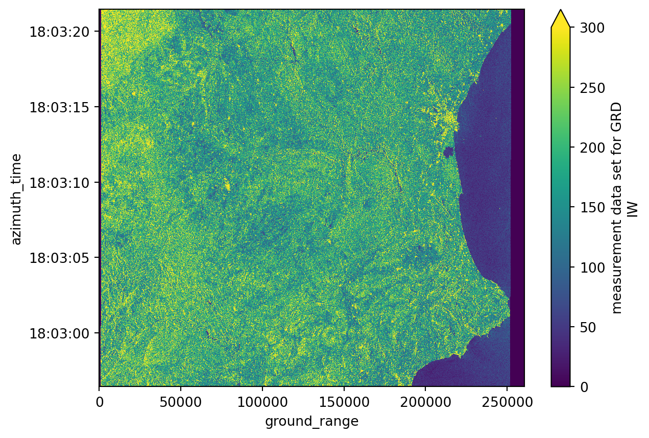

print("Azimuth time has", measurements[0].grd.shape[0], "values.")
print("Ground range has", measurements[0].grd.shape[1], "values.")

Azimuth time has 16677 values.
Ground range has 26061 values.

We use GCPs to create a spatial mask based on our bounding box, then use that mask to find the corresponding slice in SAR geometry (azimuth_time and ground_range). This approach ensures that each pixel represents the same ground location across different products, which is crucial for time series analysis.

grd = []
gcp = []

# Looping to populate the grd list with GCP-based spatial slicing
for i in range(DATASET_NUMBER):
    # Load GCPs first
    gcps = datatrees[i][datatrees[i].groups[GCP_GROUP_ID]].to_dataset()[["latitude", "longitude"]]
    
    # Create spatial mask based on bounding box
    mask = (
        (gcps.latitude < bbox[3]) & (gcps.latitude > bbox[1]) &
        (gcps.longitude < bbox[2]) & (gcps.longitude > bbox[0])
    )
    
    # Find indices where mask is True
    idx = np.where(mask == 1)
    
    if len(idx[0]) == 0 or len(idx[1]) == 0:
        continue
    
    # Build slice with offset to ensure we capture the full area
    offset = 2
    i0 = int(min(idx[0]))
    i1 = int(max(idx[0]))
    j0 = int(min(idx[1]))
    j1 = int(max(idx[1]))
    
    azimuth_time_slice = slice(max(0, i0 - offset), min(mask.shape[0], i1 + offset + 1))
    ground_range_slice = slice(max(0, j0 - offset), min(mask.shape[1], j1 + offset + 1))
    
    # Slice GCPs
    gcps_crop = gcps.isel(
        azimuth_time=azimuth_time_slice,
        ground_range=ground_range_slice
    )
    
    # Get min/max values from sliced GCPs for SAR geometry slicing
    azimuth_time_min = gcps_crop.azimuth_time.min().values
    azimuth_time_max = gcps_crop.azimuth_time.max().values
    ground_range_min = gcps_crop.ground_range.min().values
    ground_range_max = gcps_crop.ground_range.max().values
    
    # Slice GRD data using SAR geometry coordinates
    grd_crop = measurements[i].grd.sel(
        azimuth_time=slice(azimuth_time_min, azimuth_time_max),
        ground_range=slice(ground_range_min, ground_range_max)
    )
    
    # Decimate if needed (step=10 for faster processing)
    grd_crop = grd_crop.isel(
        azimuth_time=slice(None, None, 10),
        ground_range=slice(None, None, 10)
    )
    
    # Interpolate GCPs to match the sliced and decimated GRD
    gcps_crop_interp = gcps_crop.interp_like(grd_crop)
    
    # Create final mask on interpolated coordinates
    mask_2 = (
        (gcps_crop_interp.latitude < bbox[3]) & (gcps_crop_interp.latitude > bbox[1]) &
        (gcps_crop_interp.longitude < bbox[2]) & (gcps_crop_interp.longitude > bbox[0])
    )
    
    # Apply mask and drop masked values
    grd_crop = grd_crop.where(mask_2.compute(), drop=True)
    
    # We load all the variables already because we will use them in lots of future computations
    grd.append(grd_crop.load())
    gcp.append(gcps_crop_interp.load())

# Plotting the first sliced and decimated GRD product from our list 
grd[0].plot(vmax=300)
plt.title("Sliced GRD product for the area of interest")
plt.show()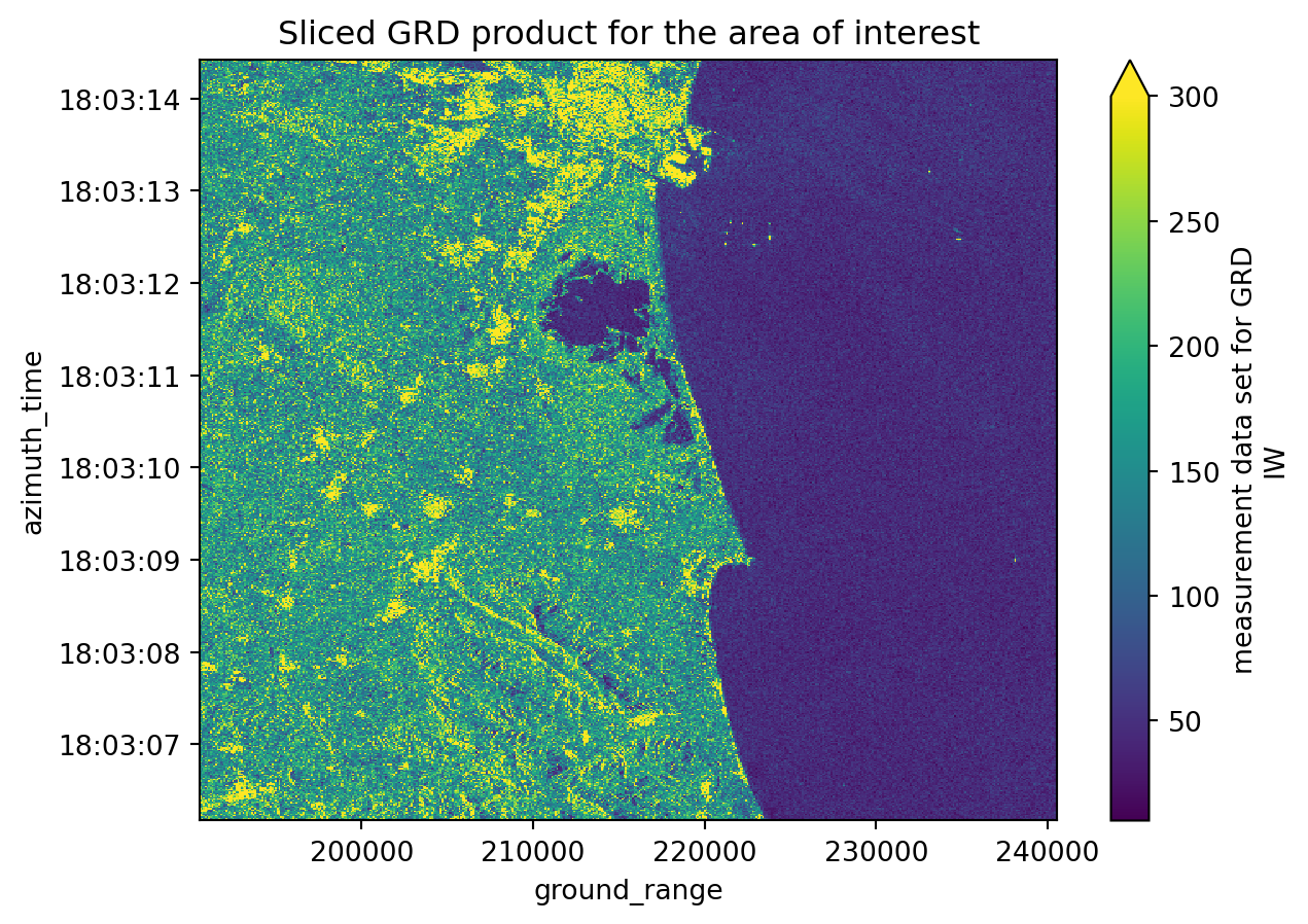

Assigning latitude and longitude coordinates

We will execute the following step to assign latitude and longitude coordinates to our datasets: 1. Creating a gcp dataset interpolated with the grd dataset; 2. Assigning the latitude and longitude coordinates to the grd dataset;

These steps are very important because we are computing a georeferenced image, which allows direct comparison with other spatial datasets. Until now, the image coordinates were expressed in azimuth_time and ground_range, which makes sense in a SAR context but not for geographical analyses.

# GCPs are now loaded and interpolated during the slicing step above
# Looping to assign the latitude and longitude coordinates to grd 
for i in range(DATASET_NUMBER):
    grd[i] = grd[i].assign_coords({"latitude": gcp[i].latitude, 
                                   "longitude": gcp[i].longitude})

# Plotting the third sliced and decimated GRD product from our list with latitude and longitude coordinates
grd[0].plot(x="longitude", y="latitude", vmax=300)
plt.title("GRD product with latitude and longitude coordinates")
plt.show()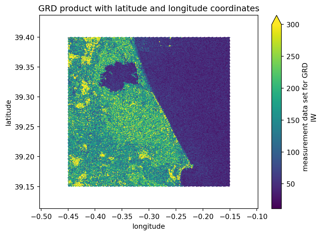

Computing backscatter

Again, the following steps are just recreating what was done before, but this time over more datasets. For further detailed information, take a look at this chapter.

Firstly we access the variables concerning the calibration values. These are the values that are going to be used for the backscatter computation.

We use manual calibration with sigma_nought instead of xarray_sentinel.calibrate_intensity() because of known issues with the product format (see forum discussion and GitLab issue). A function is created to make all the steps more automatic but you’ll see that all the procedures done inside the intensity_calibration were already explained on the previous tutorial. The manual approach uses line and pixel dimensions for interpolation, which correctly handles the calibration coefficients.

calibration = []
# Looping to populate the calibration list with only the calibration groups of each dataset on the datatree list
for i in range(DATASET_NUMBER):
    calibration.append(datatrees[i][datatrees[i].groups[CALIBRATION_GROUP_ID]].to_dataset())

def intensity_calibration(calibration, grd):
    """
    Computes the calibrated backscatter intensity from the GRD data and the calibration information.
    
    Parameters
    ----------
    calibration : xarray.Dataset
        Calibration data (e.g., sigma_nought).
    grd : xarray.DataArray
        GRD data to be calibrated.
    
    Returns
    -------
    calibrated_intensity : xarray.DataArray
        Calibrated backscatter intensity in dB.
    """
    # Accessing the sigma_nought values
    sigma_nought = calibration.sigma_nought 

    # we reacreate the sigma_nought array with line and pixel dimensions for easier interpolation
    sigma_nought_line_pixel = xr.DataArray(
        data=sigma_nought.data,
        dims=["line", "pixel"],
        coords=dict(
            line=(["line"], sigma_nought.line.values),
            pixel=(["pixel"], sigma_nought.pixel.values),
        ),
    )

    # just like for the sigma_nought, we reacreate the grd array with line and pixel dimensions for easier interpolation
    grd_line_pixel = xr.DataArray(
        data=grd.data,
        dims=["line", "pixel"],
        coords=dict(
            line=(["line"], grd.line.values),
            pixel=(["pixel"], grd.pixel.values),
        ),
    )

    # we interpolate the sigma_nought with the grd geometry
    sigma_nought_interp_line_pixel = sigma_nought_line_pixel.interp_like(grd_line_pixel, method="linear")

    sigma_nought_interp = xr.DataArray(
        data=sigma_nought_interp_line_pixel.data,
        dims=["azimuth_time", "ground_range"],
        coords=dict(
            azimuth_time=(["azimuth_time"], grd.azimuth_time.values),
            ground_range=(["ground_range"], grd.ground_range.values),
        ),
    )
    intensity = 10 * np.log10(np.maximum(((abs(grd.astype(np.float32)) ** 2) / (sigma_nought_interp**2)), 1e-10))
    return intensity

intensity = []
# Looping to populate the calibration list with only the calibration groups of each dataset on the datatree list
for i in range(DATASET_NUMBER):
    intensity.append(intensity_calibration(calibration[i], grd[i]).load())

In case we prefer to keep it more simple and calculate the intensity values with xarray_sentinel we can just uncomment the following cell and run it.

# intensity = []
# # Looping to populate the intensity list with the calibrated intensity array originated from xarray_sentinel.calibrate_intensity function
# for i in range(DATASET_NUMBER):
#     intensity.append(xarray_sentinel.calibrate_intensity(
#         grd[i], 
#         calibration[i].beta_nought, 
#         as_db=True))

# Plotting the backscatter intensity for the first dataset on the list
intensity[0].plot(x="longitude", y="latitude", vmin=-25, vmax=5)
plt.title("Computed backscatter intensity")
plt.show()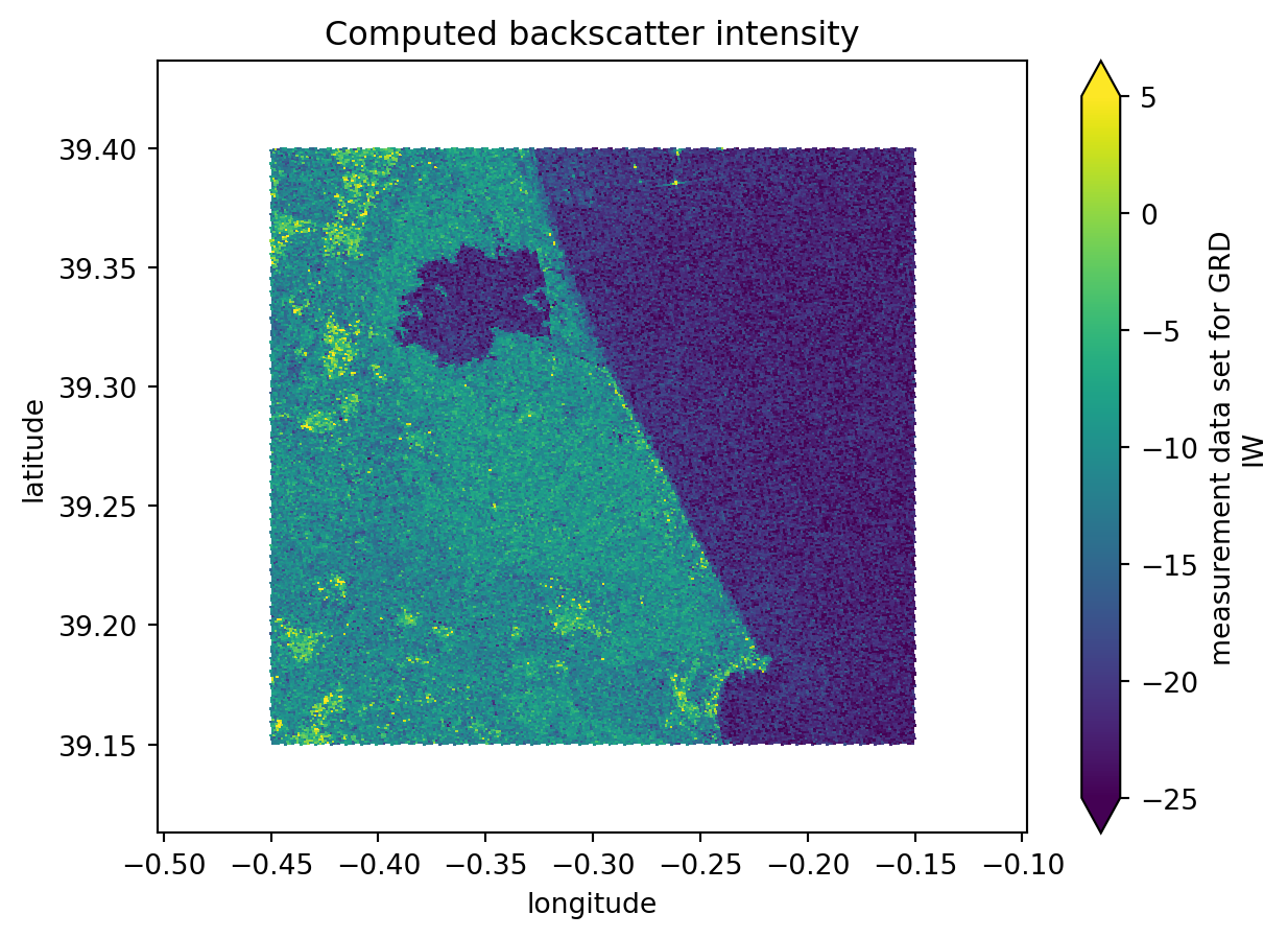

Create a datacube to prepare for time series analysis

Since we are performing a time series with .zarr, instead of analysing individual items stored in a list, we can create a combined dataset, containing all the data, stacked together by a new dimension time. Through the stacking, we are building a three-dimensional datacube.

To get values for the new dimension time, we need to extract the acquisiton dates for each product.

data = []
# Looping to populate the data list with all the acquisition dates from the datatree
for i in range(len(intensity)):
    data.append(intensity[i].azimuth_time.values[1].astype('datetime64[D]'))
data

[np.datetime64('2024-10-07'),
 np.datetime64('2024-10-19'),
 np.datetime64('2024-10-31'),
 np.datetime64('2024-11-12'),
 np.datetime64('2024-11-24'),
 np.datetime64('2024-12-06'),
 np.datetime64('2024-12-18'),
 np.datetime64('2024-12-30'),
 np.datetime64('2025-01-11'),
 np.datetime64('2025-01-23'),
 np.datetime64('2025-02-04'),
 np.datetime64('2025-02-16'),
 np.datetime64('2025-03-12'),
 np.datetime64('2025-03-24')]

Geocoding onto regular grid

In order to stack data into a time series datacube, we need to ensure that pixels across different acquisition dates correspond to the exact same ground locations. Since each Sentinel-1 GRD product has lat/lon coordinates on an irregular grid (due to SAR geometry), we need to geocode all products onto a common regular grid.

This process involves: 1. Creating a regular coordinate grid that covers all products 2. Interpolating each product’s backscatter values from its irregular lat/lon coordinates to the common regular grid 3. Stacking the geocoded products into a time series datacube

This ensures proper alignment for accurate time series analysis, where each pixel represents the same ground location across all dates.

def create_regular_grid(min_x, max_x, min_y, max_y, spatialres):
    """
    Create a regular coordinate grid given bounding box limits.
    
    Parameters
    ----------
    min_x, max_x : float
        Minimum and maximum X coordinates (e.g., longitude).
    min_y, max_y : float
        Minimum and maximum Y coordinates (e.g., latitude).
    spatialres : float
        Desired spatial resolution (in same units as x/y).
    
    Returns
    -------
    grid_x_regular : ndarray
        2D array of regularly spaced X coordinates.
    grid_y_regular : ndarray
        2D array of regularly spaced Y coordinates.
    """
    # Ensure positive dimensions and consistent spacing
    width = int(np.ceil((max_x - min_x) / spatialres))
    height = int(np.ceil((max_y - min_y) / spatialres))
    
    # Compute grid centers (half-pixel offset)
    half_pixel = spatialres / 2.0
    x_regular = np.linspace(
        min_x + half_pixel, max_x - half_pixel, width, dtype=np.float32
    )
    y_regular = np.linspace(
        min_y + half_pixel, max_y - half_pixel, height, dtype=np.float32
    )
    
    grid_x_regular, grid_y_regular = np.meshgrid(x_regular, y_regular)
    return grid_x_regular, grid_y_regular


def geocode_grd(sigma_0, grid_x_regular, grid_y_regular, time_val):
    """
    Geocode GRD backscatter from irregular lat/lon grid to regular grid.
    
    Parameters
    ----------
    sigma_0 : xarray.DataArray
        Backscatter intensity with latitude and longitude coordinates.
    grid_x_regular : ndarray
        2D array of regular X (longitude) coordinates.
    grid_y_regular : ndarray
        2D array of regular Y (latitude) coordinates.
    time_val : datetime64
        Time value for this product.
    
    Returns
    -------
    ds : xarray.Dataset
        Geocoded dataset with regular x and y coordinates.
    """
    grid_lat = sigma_0.latitude.values
    grid_lon = sigma_0.longitude.values
    
    # Set border values to zero to avoid border artifacts with nearest interpolator
    sigma_0_data = sigma_0.data.copy()
    sigma_0_data[[0, -1], :] = 0
    sigma_0_data[:, [0, -1]] = 0
    
    # Interpolate from irregular to regular grid
    interpolated_values = griddata(
        (grid_lon.flatten(), grid_lat.flatten()),
        sigma_0_data.flatten(),
        (grid_x_regular, grid_y_regular),
        method="nearest",
    )
    
    # Create xarray Dataset with regular coordinates
    ds = xr.Dataset(
        coords=dict(
            time=(["time"], [time_val]),
            y=(["y"], grid_y_regular[:, 0]),
            x=(["x"], grid_x_regular[0, :]),
        )
    )
    ds["intensity"] = (("time", "y", "x"), np.expand_dims(interpolated_values, 0))
    ds = ds.where(ds != 0)
    
    return ds


# Extract bounds from all intensity products to create common regular grid
min_lat = min([i.latitude.min().values.item() for i in intensity])
max_lat = max([i.latitude.max().values.item() for i in intensity])
min_lon = min([i.longitude.min().values.item() for i in intensity])
max_lon = max([i.longitude.max().values.item() for i in intensity])

# Create common regular grid (resolution: 0.0001 degrees ≈ 11 meters)
grid_x_regular, grid_y_regular = create_regular_grid(
    min_lon, max_lon, min_lat, max_lat, 0.0001
)

Now we geocode all products onto the common regular grid and stack them into a time series datacube. Each pixel now corresponds to the exact same ground location across all acquisition dates, enabling accurate time series analysis.

# Geocode all products onto the common regular grid
geocoded = []
for i in range(len(intensity)):
    geocoded.append(geocode_grd(intensity[i], grid_x_regular, grid_y_regular, data[i]))

# Create the data cube by stacking all geocoded products
intensity_data_cube = xr.concat(geocoded, dim="time").sortby("time")

# There is a new dimension coordinate (time) 
intensity_data_cube

Flood mapping and time series analysis

The last step is to perform the time series and flood mapping analysis.

Simple visualisation of all datasets selected

First, we can plot all the datasets simply to create a visualisation of the flood. In addition to these plots, we are also plotting a chosen latitude and longitude point (as defined at beginning of this tutorial). The coordinate serves as a measure of comparison between all the datasets and from within different analysis methods.

When we look over all the items plotted, we can clearly see that the significant flood event happened between the 19th and the 31st of October (it occurred on the 29th of October 2024).

Additionally, we can see that the backscatter displaying the water presence was only going back to normal ranges around mid-February 2025.

cols = 4    # setting up column number
rows = int(np.ceil(len(geocoded) / cols))  # setting up row number according to column number
fig, axes = plt.subplots(rows, cols, figsize=(4*cols, 4*rows))  
axes = axes.flatten()  

for i in range(len(geocoded)):
    ax = axes[i]
    intensity_data_cube.isel(time=i).intensity[::4, ::4].plot(    # plotting all the datasets stored in the data cube
        x="x", y="y",
        vmin=-25, vmax=5,
        ax=ax,  
        add_colorbar=False  
    )
    ax.scatter(TARGET_LONG, TARGET_LAT, color="red", marker="o", s=10, label="Selected Point")  # also plotting the known point defined before
    ax.legend(loc="upper right")

for j in range(i+1, len(axes)):
    axes[j].axis('off')     # to avoid having empty cells

plt.tight_layout()
plt.show()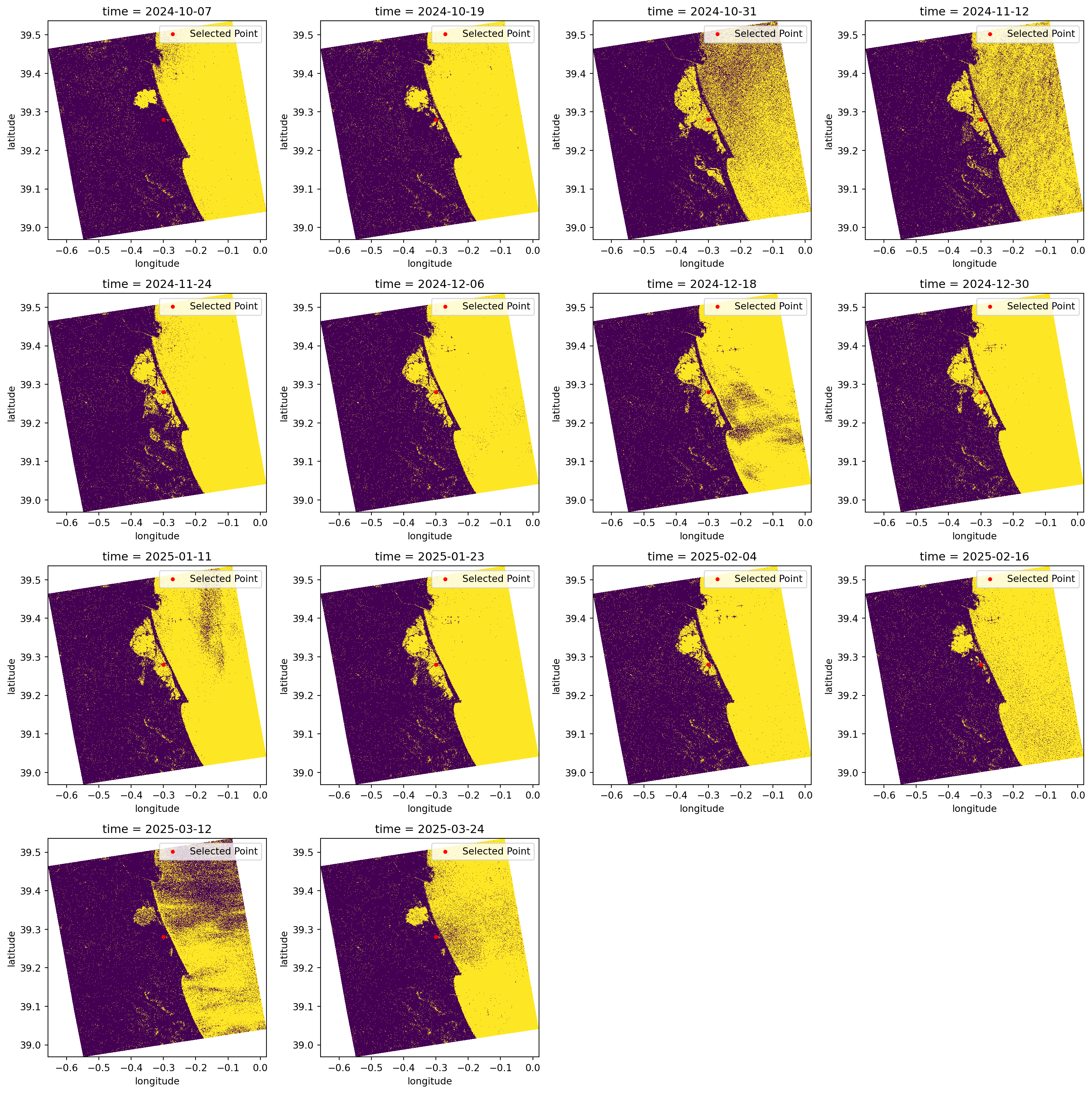

Create a flood map based on threshold values

It is known through literature and other sources that water appears as darker pixels, typically with values lower than -15 dB. This is a very good method for identifying water because separating the pixels within this threshold value will give us almost a True and False map for pixels which are greater or smaller than the defined threshold.

In the plots below, we classify the pixels with backscatter values equal to or lower than -15 in yellow. Conversely, in purple, we see the pixels that have backscatter values greater than -15.

This type of visualisation allows us to easily identify flooded and non-flooded areas.

fig, axes = plt.subplots(rows, cols, figsize=(4*cols, 4*rows))  
axes = axes.flatten()  

for i in range(len(geocoded)):
    ax = axes[i]
    water_mask = (intensity_data_cube.isel(time=i).intensity[::4, ::4] <= WATER_THRESHOLD_DB)     # defining the water mask from the threshold
    water_mask.plot(        # plotting all the water masks 
        x="x", y="y",
        ax=ax,  
        add_colorbar=False  
    )
    ax.scatter(TARGET_LONG, TARGET_LAT, color="red", marker="o", s=10, label="Selected Point") # again plotting the known point defined before
    ax.legend(loc="upper right")

for j in range(i+1, len(axes)):
    axes[j].axis('off')

plt.tight_layout()
plt.show()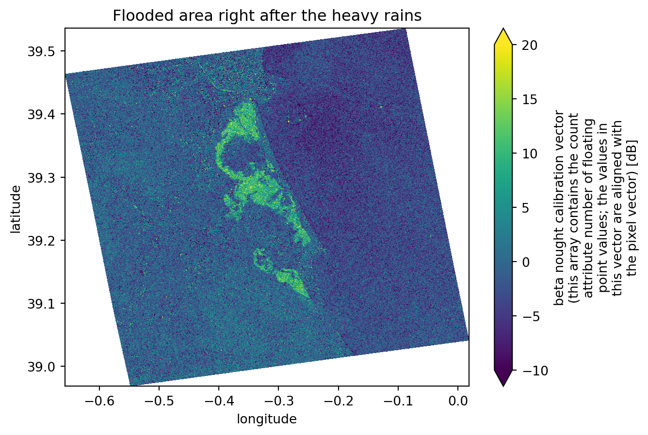

Create a map showing differences between two images

Knowing the exact flood date, which we have, and from the images plotted previously, we can easily see that the second image is the one right before the flood event and that the third image is the one directly after it. These two images show significant differences in the flooded areas and backscatter values, ranging from -5 dB (in the image before the event) to -20 dB (in the image directly after the event).

For this reason, when we compute the difference between the two images, we will mostly get: - Values around 0 dB for areas that did not change - Values ranging from -15 dB to -20 dB in the precise flooded areas.

This is an excellent way to determine precisely which areas were flooded. As we are comparing an image from before the event with another one taken at the highest possible flooding point, the differences between them will be extreme.

dif = (intensity_data_cube.isel(time=1).intensity - intensity_data_cube.isel(time=2).intensity)   # computing the difference between third and second dataset
dif.plot(x="x", y="y", vmin=-10, vmax=20)
plt.title("Flooded area right after the heavy rains")
plt.show()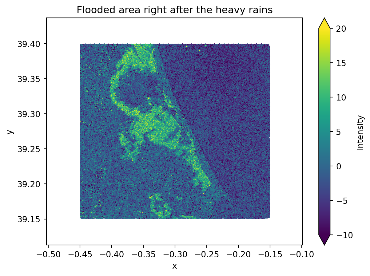

Create a time-series plot of one location within the flood

Taking advantage of the data cube we have created over a new time dimension, it is much easier to plot the data over this new dimension, as in a time series plot.
As our data now shares same dimensions and shape, we can choose to plot a backscatter analysis over the specific latitude and longitude point we defined earlier.

As these coordinates might not be exactly the ones shown on the dimension values, we need to perform some operations to find the closest values to the desired coordinates.
We will now change the latitude and longitude coordinate values and see how the corresponding azimuth_time and ground_range values and indexes change.

# Find how far each pixel's coordinates are from the target point
abs_error = np.abs(intensity_data_cube.y - TARGET_LAT) + np.abs(intensity_data_cube.x - TARGET_LONG)  

# Get the indexes of the closest point
i, j = np.unravel_index(np.argmin(abs_error.values), abs_error.shape)
y_index = i
x_index = j

# Get the coordinate values of the closest point
y_value = intensity_data_cube.y[i].values
x_value = intensity_data_cube.x[j].values

print("Nearest y (latitude):", y_value, ", with index:", y_index)
print("Nearest x (longitude):", x_value, ", with index:", x_index)

# Slice the data cube in order to get only the pixel that corresponds to the target point
target_point = intensity_data_cube.isel(y=y_index, x=x_index).intensity

Nearest y (latitude): 39.280018 , with index: 1672
Nearest x (longitude): -0.3000041 , with index: 2029

Now we can plot the data cube, showing the backscatter intensity over the target point we defined earlier. Since the datasets are stacked along the time dimension, it becomes much easier to plot the evolution of water backscatter at a specific location. This provides an effective way to monitor the flooding status at that point.

We can also add a line representing the water threshold we defined. Any point with a backscatter value below this threshold will be classified as water, thus flooded.

# Plot the sliced data cube
target_point.plot(label='Time series backscatter') 

x = target_point[target_point.dims[0]].values   # getting the x axis values (time)
y = target_point.values                         # getting the y axis values (backscatter intensity)

# Creating the trend line
x_num = np.arange(len(x))   
z = np.polyfit(x_num, y, 6)
p = np.poly1d(z)

plt.plot(x, p(x_num), 'r--', label='Trend line')
plt.plot(x, [-15] * len(x), 'g--', label='Flood threshold')
plt.legend()
plt.show()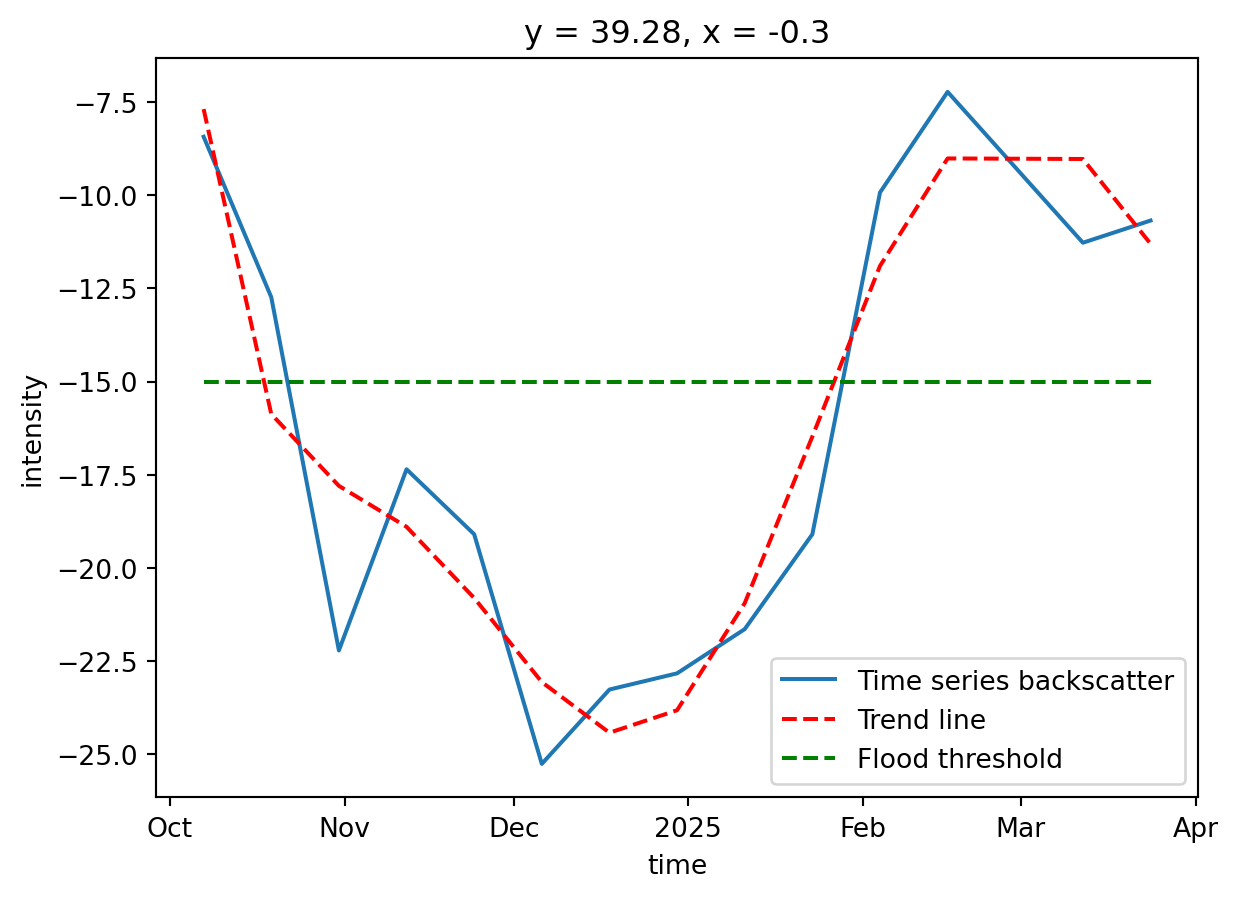

Challenges

While using the optimised .zarr format saves a lot of time and makes creating workflows relatively simple and achievable, there are still a few challenges to handle and to keep in mind:

Sentinel-1 GRD Data Availability: For Sentinel-1 GRD, most of the datasets are not yet available on the STAC catalogue. This makes searching and data handling harder because, in the end, only a few products are correctly converted.
Backscatter Computation: The xarray_sentinel library has known issues with certain product formats, requiring manual calibration using sigma_nought with line and pixel dimension interpolation. This tutorial demonstrates the correct manual calibration approach.
Geocoding: Proper geocoding onto a regular grid is essential for accurate time series analysis. This tutorial uses scipy.interpolate.griddata to geocode products from irregular SAR geometry coordinates to a common regular grid, ensuring pixels correspond to the same ground locations across all dates.
Terrain Correction: With the available libraries, it is very difficult to perform geometric and radiometric terrain correction. The existing tools that support the .zarr format are not yet fully operational and do not accept the format as it is.

Conclusion

The .zarr format is particularly well suited for hazard analysis because it enables multiple datasets to be combined into a single structure, either as a data cube or as a list of datatrees. This makes it ideal for rapid, multi-temporal, and multi-spatial monitoring. Unlike the .SAFE format, which required downloading entire products, .zarr only loads the specific groups needed, while the rest is accessed on the fly. As a result, both data handling and subsequent operations are much faster and more efficient. The .load() helps a lot on these situations.

Although the ecosystem for .zarr is still evolving, there are already promising developments. In the past, .SAFE products could be fully processed on applications like SNAP, but similar completeness has not yet been reached for .zarr. Nevertheless, libraries such as xarray_sentinel and are beginning to cover essential SAR operations. This potential is illustrated in the Valencia flood case study, where Sentinel-1 backscatter sensitivity to water enabled clear mapping of flood extent and duration. The same workflow can be adapted to other flood events by adjusting the relevant thresholds and parameters to match local conditions.

What’s next?

In the following notebook we will explore a new approach to the EOPF Zarr format.
We will follow step by step the creation of Overviews, taking as a starting point the existing EOPF Zarr format structure and taking it to the next level!