Comparisons of SAFE vs Zarr in R
By: @sharlagelfand | SparkGeo
Introduction
Prior to the introduction of EOPF’s Zarr, the ESA’s Copernicus data was published and distributed using the Standard Archive Format for Europe (SAFE). Sentinel scenes were downloaded as zip archives, containing several files as well as an XML manifest. In order to access any scene data, the entire zip archive had to be downloaded, which could be quite inefficient.
Zarr is optimised for efficient data retrieval; arrays are segmented into one or more chunks, and a single Sentinel scene could potentially be across several chunks. A data consumer can choose to download only the chunks required for their use case, rather than the entire zip archive. There is no need to download all data before processing it, and data can be lazy-loaded so that it is only downloaded when required. The Comparisons section shows how this is more efficient in terms of both network bandwidth and compute resources.
The following chapter will contrast the processes for working with EOPF Zarr versus the SAFE format, showing that Zarr takes less code, time, and downloads less data.
We recommend reviewing the previous R tutorials if you have not done so already:
What we will learn
- 🗂 How to extract Copernicus data in the Standard Archive Format for Europe (SAFE) format.
- 📊 How to compare metrics such as code runtime and download size between SAFE and Zarr.
Prerequisites
An R environment is required to follow this tutorial, with R version >= 4.5.0. For local development, we recommend using either RStudio or Positron and making use of RStudio projects for a self-contained coding environment.
We will use the following packages in this tutorial:
rstac(for accessing the STAC catalog)tidyverse(for data manipulation)terra(for working with spatial data in raster format)stars(for reading, manipulating, and plotting spatiotemporal data)httr2(for working with APIs)xml2(for accessing metadata from SAFE files)fs(for accessing file locations and sizes)lobstr(for calculating the size of objects within R)
You can install these packages directly from CRAN. Note that xml2 is a part of tidyverse, so it does not need to be installed separately, but it will be loaded separately.
# install.packages("rstac")
# install.packages("tidyverse")
# install.packages("stars")
# install.packages("terra")
# install.packages("httr2")
# install.packages("fs")
# install.packages("lobstr")
We will also use the Rarr package (version >= 1.10.0) to read Zarr data. It must be installed from Bioconductor, so first install the BiocManager package:
# install.packages("BiocManager")Then, use this package to install Rarr:
# BiocManager::install("Rarr")Finally, load the packages into your environment:
library(rstac)
library(tidyverse)
library(stars)
library(terra)
library(httr2)
library(fs)
library(lobstr)
library(xml2)
library(Rarr)
Zarr example
This example shows how to access the 60-metre resolution quicklook of a Sentinel-2 mission, explored in more detail the tutorial More examples analysing EOPF STAC Zarr data with R.
We set up zarr_start and zarr_end to time the data retrieval and visualisation process, for comparison to the SAFE process later on.
zarr_start <- Sys.time()

item_id <- "S2B_MSIL2A_20250530T101559_N0511_R065_T32TPT_20250530T130924"

s2_l2a_item <- stac("https://stac.core.eopf.eodc.eu/") |>
  collections(collection_id = "sentinel-2-l2a") |>
  items(feature_id = item_id) |>
  get_request()

s2_l2a_product <- s2_l2a_item |>
  assets_select(asset_names = "product")

s2_l2a_product_url <- s2_l2a_product |>
  assets_url()

zarr_store <- s2_l2a_product_url |>
  zarr_overview(as_data_frame = TRUE) |>
  mutate(array = str_remove(path, s2_l2a_product_url)) |>
  relocate(array, .before = path)

r60m_tci <- zarr_store |>
  filter(array == "/quality/l2a_quicklook/r60m/tci") |>
  pull(path) |>
  read_zarr_array()

r60m_tci <- r60m_tci |>
  aperm(c(2, 3, 1)) |>
  rast()

r60m_tci |>
  plotRGB()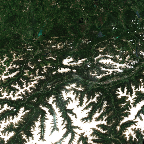
zarr_end <- Sys.time()SAFE example
The following example accesses the same 60-metre quicklook image as the example above, using SAFE instead of EOPF Zarr.
This example also requires authentication to the SAFE STAC API. You need a Copernicus Dataspace account, and to store your username and password in the environment variables CDSE_USERNAME and CDSE_PASSWORD (using e.g. usethis::edit_r_environ() to set these).
We then use this to generate a token:
token <- oauth_client(
  id = "cdse-public",
  token_url = "https://identity.dataspace.copernicus.eu/auth/realms/CDSE/protocol/openid-connect/token"
) |>
  oauth_flow_password(
    username = Sys.getenv("CDSE_USERNAME"),
    password = Sys.getenv("CDSE_PASSWORD")
  )

token
## <httr2_token>
## * token_type : "Bearer"
## * access_token : <REDACTED>
## * expires_at : "2026-03-06 16:57:16"
## * refresh_token : <REDACTED>
## * refresh_expires_in: 3600
## * not-before-policy : 0
## * session_state : "0b942e6f-0b09-cc0b-5d55-f543d6d9e12e"
## * scope : "AUDIENCE_PUBLIC openid email profile ondemand_processing user-context"This token will be used for accessing SAFE data. The token object contains the token itself and, as you can see, when it expires (30 minutes after generation).
To access the SAFE data, we first get the STAC item from the Sentinel-2 collection. Its ID is the same as in the EOPF Sample Service STAC catalog example, with the suffix .SAFE. We’ll also set up timing how long this process takes, in safe_start.
safe_start <- Sys.time()

safe_item <- stac("https://stac.dataspace.copernicus.eu/v1") |>
  collections(collection_id = "sentinel-2-l2a") |>
  items(feature_id = item_id) |>
  get_request()

safe_item
## ###Item
## - id: S2B_MSIL2A_20250530T101559_N0511_R065_T32TPT_20250530T130924
## - collection: sentinel-2-l2a
## - bbox: xmin: 10.31189, ymin: 46.83277, xmax: 11.80285, ymax: 47.84592
## - datetime: 2025-05-30T10:15:59.024Z
## - assets:
## AOT_10m, AOT_20m, AOT_60m, B01_20m, B01_60m, B02_10m, B02_20m, B02_60m, B03_10m, B03_20m, B03_60m, B04_10m, B04_20m, B04_60m, B05_20m, B05_60m, B06_20m, B06_60m, B07_20m, B07_60m, B08_10m, B09_60m, B11_20m, B11_60m, B12_20m, B12_60m, B8A_20m, B8A_60m, Product, SCL_20m, SCL_60m, TCI_10m, TCI_20m, TCI_60m, WVP_10m, WVP_20m, WVP_60m, thumbnail, safe_manifest, granule_metadata, inspire_metadata, product_metadata, datastrip_metadata
## - item's fields:
## assets, bbox, collection, geometry, id, links, properties, stac_extensions, stac_version, typeThe relevant asset is “Product”:
safe_item |>
  items_assets()
## [1] "AOT_10m" "AOT_20m" "AOT_60m"
## [4] "B01_20m" "B01_60m" "B02_10m"
## [7] "B02_20m" "B02_60m" "B03_10m"
## [10] "B03_20m" "B03_60m" "B04_10m"
## [13] "B04_20m" "B04_60m" "B05_20m"
## [16] "B05_60m" "B06_20m" "B06_60m"
## [19] "B07_20m" "B07_60m" "B08_10m"
## [22] "B09_60m" "B11_20m" "B11_60m"
## [25] "B12_20m" "B12_60m" "B8A_20m"
## [28] "B8A_60m" "Product" "SCL_20m"
## [31] "SCL_60m" "TCI_10m" "TCI_20m"
## [34] "TCI_60m" "WVP_10m" "WVP_20m"
## [37] "WVP_60m" "thumbnail" "safe_manifest"
## [40] "granule_metadata" "inspire_metadata" "product_metadata"
## [43] "datastrip_metadata"We can select its URL for accessing the data:
safe_url <- safe_item |>
  assets_select(asset_names = "Product") |>
  assets_url()

safe_url
## [1] "https://download.dataspace.copernicus.eu/odata/v1/Products(fa3a0848-1568-4dc4-9ecb-dabecf23bd4b)/$value"The following code sets up the API request via httr2’s request(), adding in the token as a Bearer token so that we are authenticated and have permission to access the data. Then, we add error handling, which is informative in case the token has expired; in which case, the above OAuth token generation code should be rerun. Then, we perform the request (via req_perform()) and save it to a ZIP file, stored in safe_zip.
safe_dir <- tempdir()
safe_zip <- paste0(safe_dir, "/", item_id, ".zip")

request(safe_url) |>
  req_auth_bearer_token(token$access_token) |>
  req_error(body = \(x) resp_body_json(x)[["message"]]) |>
  req_perform(path = safe_zip)
## <httr2_response>
## GET https://download.dataspace.copernicus.eu/odata/v1/Products(fa3a0848-1568-4dc4-9ecb-dabecf23bd4b)/$value
## Status: 200 OK
## Content-Type: application/zip
## Body: On disk (1259528508 bytes)We need to unzip the file and find the manifest file, which contains information on where different data sets are.
unzip(safe_zip, exdir = safe_dir)

safe_unzip_dir <- paste0(safe_dir, "/", item_id, ".SAFE")

safe_files <- tibble(path = dir_ls(safe_unzip_dir)) |>
  mutate(file = basename(path)) |>
  relocate(file, .before = path)

safe_files
## # A tibble: 8 × 2
## file path
## <chr> <fs::path>
## 1 DATASTRIP …DATASTRIP
## 2 GRANULE …E/GRANULE
## 3 HTML …SAFE/HTML
## 4 INSPIRE.xml …SPIRE.xml
## 5 MTD_MSIL2A.xml …SIL2A.xml
## 6 S2B_MSIL2A_20250530T101559_N0511_R065_T32TPT_20250530T130924-… …24-ql.jpg
## 7 manifest.safe …fest.safe
## 8 rep_info …/rep_infomanifest_location <- safe_files |>
filter(file == "manifest.safe") |>
pull(path)We then read in the manifest file, and find the location of the 60-metre resolution data.
manifest <- read_xml(manifest_location)

safe_r60m_quicklook_location <- manifest |>
  xml_find_first(".//dataObject[@ID='IMG_DATA_Band_TCI_60m_Tile1_Data']/byteStream/fileLocation") |>
  xml_attr("href")

safe_r60m_quicklook_location
## [1] "./GRANULE/L2A_T32TPT_A042991_20250530T101708/IMG_DATA/R60m/T32TPT_20250530T101559_TCI_60m.jp2"Which we can then read in and visualize:
safe_r60m_quicklook_location <- paste0(safe_unzip_dir, str_remove(safe_r60m_quicklook_location, "\\."))

r60m_tci_safe <- read_stars(safe_r60m_quicklook_location) |>
  st_rgb()

r60m_tci_safe |>
  plot()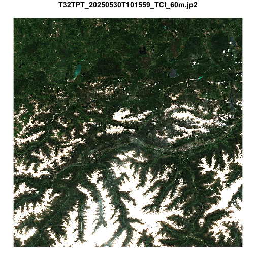
safe_end <- Sys.time()Comparisons
To contrast with the Zarr example, we’ll look at how long the processes took, how large the objects are, and how much data was saved to disk.
First, to compare the time:
zarr_end - zarr_start## Time difference of 31.67 secssafe_end - safe_start## Time difference of 10.88 minstime_diff <- (safe_time_numeric * 60) - zarr_time_numeric
time_diff_min <- round(time_diff / 60, 2)The EOPF Zarr example took 31.67 seconds, while the SAFE example took 10.88 minutes—a difference of over 10 minutes.
We can also compare the size of the objects in R:
obj_size(r60m_tci)## 9.69 MBobj_size(r60m_tci_safe)## 45.99 MBThe object from the SAFE example is nearly 5 times larger than the EOPF Zarr object.
Finally, the SAFE example requires saving the entire archive to disk, while nothing is saved to disk in the Zarr example. The size of the full archive is:
file_size(safe_zip)## 1.17Gwhile the size of the manifest file and the 60-metre resolution quicklook file are:
file_size(manifest_location)## 67.3Kfile_size(safe_r60m_quicklook_location)## 3.57MSo, of the 1.17G saved to disk, only 0.3% was actually used.
To summarise:
| Format | Time | Downloaded to disk | Download used | Object size |
|---|---|---|---|---|
| EOPF Zarr | 31.67 secs | — | — | 9.69 MB |
| SAFE | 10.88 mins | 1.17G | 0.3% | 45.99 MB |
Optimisations
The transition from SAFE to EOPF Zarr presents opportunities for optimisations that may affect the data provider (ESA), the data consumer, or both.
Chunk Size
Zarr supports configurable chunk sizes for array data. A Zarr store may contain many n-dimensional arrays and each can support a unique chunk size. Each array will comprise one or more chunks of this size.
Chunk size is determined by the data provider and, ideally, is configured such that the chunks downloaded by a data consumer to satisfy a given use-case include minimal extraneous data.
STAC Metadata and Zarr
The relationship between STAC metadata and Zarr stores is a source of discussion and a number of different strategies are available, each with differing advantages and disadvantages. Additional context on this subject can be found in the Cloud-Optimized Geospatial Formats Guide.
The approach adopted for STAC metadata in the EOPF Sample STAC Service most closely aligns to the many smaller Zarr stores approach.
Memory Limitations
If a use case requires more memory than the data consumer can support, even after optimisation efforts, it may be necessary to use a cloud-hosted compute environment with access to a larger pool of compute resources.
What’s next?
In the following notebook we will explore the use of rarr, terra and stars to showcase retrieval of Sentinel-2 L2A Products with R.