Sentinel-1 SAR Flood Detection and Mapping Using Change Detection

By: @HillaryKoros | GIS & AI Researcher , DevOps Engineer

Introduction

East Africa faces devastating seasonal flooding that displaces hundreds of thousands of people, destroys crops, and damages critical infrastructure. Kenya’s Tana River basin β€” the country’s longest river system β€” experiences severe flooding during the short rains (October–December) when intense precipitation overwhelms drainage capacity across the coastal lowlands.

This notebook implements the UN-SPIDER Recommended Practice for SAR flood mapping β€” a change detection approach comparing pre-flood and post-flood imagery β€” adapted from Google Earth Engine to run entirely on EOPF Zarr data via cloud-native access. We use a matched Sentinel-1 image pair captured just 12 days apart β€” before and after the documented flood event β€” to map the inundation extent and assess its impact.

🚨 The Event: On November 22–23, 2025, heavy rains caused the Tana River to burst its banks, flooding communities across Tana River County and affecting approximately 4,900 households. Families were displaced, farmland submerged, and access roads cut off β€” a scenario that repeats with increasing frequency as flash-flood events in the region have risen 40% in the last decade.

⚠️ The Challenge: During active flood events, persistent cloud cover renders optical satellite imagery useless. Decision-makers need flood extent maps within hours, not days. Traditional ground surveys are impossible when roads are submerged.

βœ… The Solution: Synthetic Aperture Radar (SAR) from the Sentinel-1 mission penetrates clouds, operates day and night, and detects water on the ground by measuring how radar signals bounce off the surface. When radar hits calm water, it reflects away from the sensor (specular reflection), producing characteristically low backscatter that contrasts sharply with dry land.

What we will learn

  • πŸ›°οΈ EOPF STAC + Zarr Access: Discover and load Sentinel-1 GRD data from the EOPF cloud-native catalog β€” no bulk downloads needed

  • πŸ“‘ SAR Processing Pipeline: Radiometric calibration (DN β†’ σ⁰ dB), georeferencing via GCPs, and speckle filtering.

  • 🌊 Flood Detection: Ratio-based change detection following the UN-SPIDER methodology, with threshold tuning and refinement

  • πŸ“Š Impact Assessment: Overlay flood extent on population density and land cover to estimate who and what is affected

Prerequisites

Phase What we do Why it matters
1 Search EOPF STAC for matched Sentinel-1 GRD pairs Same orbit + sensor ensures valid comparison
2 Calibrate, georeference, and filter radar imagery Convert raw data to physically meaningful backscatter
3 Ratio-based change detection with threshold tuning Identify newly inundated areas between pre- and post-flood
4 Overlay flood extent on population and land cover Translate maps into actionable damage estimates

πŸ“ Study area: Tana River floodplain, Kenya β€” centered near Hola (40.05Β°E, 1.50Β°S)
πŸ“… Event: Tana River flooding, November 22–23, 2025
πŸ›°οΈ Comparison: November 11, 2025 (pre-flood) vs November 23, 2025 (flood day) β€” 12-day repeat cycle

pystac-client
STAC catalog search

zarr
Cloud-native data

numpy / scipy
Arrays & filtering

matplotlib
Static maps

folium
Interactive maps

πŸ“š Background reading: - UN-SPIDER: Recommended Practice for SAR Flood Mapping β€” the methodology we adapt - EOPF 101 Book β€” introduction to the EOPF ecosystem - Sentinel-1 User Guide β€” SAR fundamentals and product specifications

πŸ“‘ Workflow at a Glance

πŸ›°οΈ
Phase 1
STAC Discovery
Find matched S1 pairs
via EOPF catalog
βš™οΈ
Phase 2
SAR Processing
Calibrate, georeference
& filter speckle
🌊
Phase 3
Flood Detection
Ratio change detection
& refinement
πŸ“Š
Phase 4
Impact Assessment
Population, cropland
& urban exposure

πŸ“ Tana River, Kenya πŸ“… Nov 22–23, 2025 flood event πŸ›°οΈ 12-day S1 repeat pair ☁️ Cloud-native EOPF Zarr


Import libraries

import subprocess
import sys
import warnings
import folium 
import matplotlib.patches as mpatches 
import matplotlib.pyplot as plt 
import numpy as np  
import zarr 
from IPython.display import display  
from matplotlib.colors import ListedColormap  
from pystac_client import Client  
from scipy.interpolate import griddata  
from scipy.ndimage import label as ndlabel 
from scipy.ndimage import uniform_filter, zoom 

warnings.filterwarnings('ignore')

print("Dependencies installed and libraries loaded.")
Dependencies installed and libraries loaded.

βš™οΈ Configuration

All parameters in one place. The DIFFERENCE_THRESHOLD of 1.25 comes from the UN-SPIDER Recommended Practice.

πŸŽ›οΈ Threshold tuning: The threshold typically requires several rounds of testing to achieve the best results for a given scene. Factors like terrain type, soil moisture, vegetation density, and flood severity all affect the optimal value. We recommend using the sensitivity analysis in Section 3.5 to evaluate how flood extent changes across a range of thresholds, then adjusting based on visual inspection and local knowledge. Values between 1.1–2.0 are common in the literature.

# EOPF STAC endpoint
STAC_API_URL = "https://stac.core.eopf.eodc.eu"
COLLECTION_ID = "sentinel-1-l1-grd"

# Study area: Tana River floodplain, Kenya
# Center: Hola/Tana River (-1.50Β°N, 40.05Β°E)
BBOX = [39.5, -2.1, 40.6, -0.9]

# Target center for spatial subset β€” Tana River near Hola
TARGET_LAT = -1.502380
TARGET_LON = 40.052577

# Time periods β€” targeting the Nov 22-23 Tana River flood event
# S1A same orbit pair, 12 days apart, covers the floodplain
BEFORE_PERIOD = "2025-11-11T15:39:00Z/2025-11-11T15:41:00Z"  # Pre-flood
AFTER_PERIOD  = "2025-11-23T15:39:00Z/2025-11-23T15:41:00Z"  # Flood day

# SAR processing parameters (UN-SPIDER methodology)
POLARIZATION = "vh"            # VH preferred: sensitive to surface roughness changes
DIFFERENCE_THRESHOLD = 1.25    # UN-SPIDER Recommended Practice default (tune with Section 3.5)
SPECKLE_KERNEL = 7             # Focal mean filter size (~70m smoothing window)
MIN_FLOOD_CLUSTER = 15         # Min connected pixels to retain (removes isolated noise)

# Spatial subset for efficient processing
SUBSET_SIZE = 4000             # 4000Γ—4000 px = 40Γ—40 km at 10m GRD resolution

print(f"πŸ“ Study area: {BBOX}")
print(f"🎯 Target center: {TARGET_LAT}°N, {TARGET_LON}°E (Tana River, near Hola)")
print(f"πŸ“‘ Polarization: {POLARIZATION.upper()} | Threshold: {DIFFERENCE_THRESHOLD} (UN-SPIDER)")
print(f"πŸ”§ Speckle kernel: {SPECKLE_KERNEL} | Min cluster: {MIN_FLOOD_CLUSTER} px")
print(f"πŸ“ Processing subset: {SUBSET_SIZE}Γ—{SUBSET_SIZE} pixels ({SUBSET_SIZE*10/1000:.0f}Γ—{SUBSET_SIZE*10/1000:.0f} km)")
πŸ“ Study area: [39.5, -2.1, 40.6, -0.9]
🎯 Target center: -1.50238°N, 40.052577°E (Tana River, near Hola)
πŸ“‘ Polarization: VH | Threshold: 1.25 (UN-SPIDER)
πŸ”§ Speckle kernel: 7 | Min cluster: 15 px
πŸ“ Processing subset: 4000Γ—4000 pixels (40Γ—40 km)

Helper functions

The workflow uses the following core functions, each defined in context where first used:

Function Purpose Defined in
load_grd_subset() Load spatial subset of S1 GRD from EOPF Zarr Phase 2.1
calibrate_to_sigma0_db() Radiometric calibration (DN β†’ σ⁰ dB) Phase 2.2
georeference_subset() GCP interpolation for lat/lon coordinates Phase 2.3
plot_sar() Georeferenced SAR visualization Phase 2.4
speckle_filter() Focal mean filter in linear domain Phase 2.5
refine_flood() Connected component noise removal Phase 3.2

πŸ›°οΈ Phase 1: Data Acquisition

1.1 Searching the EOPF STAC Catalog

For change detection to work, we need images from the same orbit and sensor so the viewing geometry is identical. We search for Sentinel-1C ascending passes over our study area β€” one from before the November 22–23 flood event and one from after.

catalog = Client.open(STAC_API_URL)
print(f"Connected to: {STAC_API_URL}")
print(f"Collections: {[c.id for c in catalog.get_collections()]}\n")

# Search for matched image pair
def search_items(period):
    results = catalog.search(
        collections=[COLLECTION_ID], bbox=BBOX,
        datetime=period, max_items=10
    )
    # Filter to images that cover the Tana River floodplain (target point)
    items = []
    for i in results.items():
        # Check if image bbox contains our target point
        if (i.bbox[0] <= TARGET_LON <= i.bbox[2] and
            i.bbox[1] <= TARGET_LAT <= i.bbox[3]):
            items.append(i)
    return items

before_items = search_items(BEFORE_PERIOD)
after_items = search_items(AFTER_PERIOD)

print(f"Found {len(before_items)} before and {len(after_items)} after images covering target\n")

before_item = before_items[0]
after_item = after_items[0]

print("SELECTED IMAGE PAIR (same orbit, same sensor):")
print(f"  BEFORE:  {before_item.id}")
print(f"    Date: {before_item.datetime.strftime('%Y-%m-%d %H:%M')} | Bbox: {[round(x,1) for x in before_item.bbox]}")
print(f"  AFTER:   {after_item.id}")
print(f"    Date: {after_item.datetime.strftime('%Y-%m-%d %H:%M')} | Bbox: {[round(x,1) for x in after_item.bbox]}")
print(f"  Gap: {(after_item.datetime - before_item.datetime).days} days")
print(f"  Assets: {list(before_item.assets.keys())}")
Connected to: https://stac.core.eopf.eodc.eu
Collections: ['sentinel-2-l2a', 'sentinel-1-l1-grd', 'sentinel-1-l1-slc', 'sentinel-3-olci-l1-efr', 'sentinel-3-slstr-l2-lst', 'sentinel-1-l2-ocn', 'sentinel-3-olci-l2-lfr', 'sentinel-3-slstr-l1-rbt', 'sentinel-3-olci-l1-err', 'sentinel-3-olci-l2-lrr', 'sentinel-2-l1c', 'sentinel-3-slstr-l2-frp']

Found 1 before and 1 after images covering target

SELECTED IMAGE PAIR (same orbit, same sensor):
  BEFORE:  S1A_IW_GRDH_1SDV_20251111T153956_20251111T154021_061831_07BAD6_E493
    Date: 2025-11-11 15:40 | Bbox: [38.7, -2.4, 41.2, -0.4]
  AFTER:   S1A_IW_GRDH_1SDV_20251123T153955_20251123T154020_062006_07C1A9_E682
    Date: 2025-11-23 15:40 | Bbox: [38.7, -2.4, 41.2, -0.4]
  Gap: 11 days
  Assets: ['vh', 'vv', 'product', 'noise-vh', 'noise-vv', 'calibration-vh', 'calibration-vv', 'zipped_product', 'product_metadata']

1.2 Verify Study Area Coverage

Before processing, let’s confirm our selected images cover the Tana River floodplain. The interactive map below shows: - Red box: Our bounding box search area - Blue boxes: Footprints of the selected before/after images
- Green marker: Our target center point on the Tana River

# Interactive map to verify study area and image coverage
m_verify = folium.Map(location=[TARGET_LAT, TARGET_LON], zoom_start=9, tiles='OpenStreetMap')

# Satellite basemap
folium.TileLayer(
    tiles='https://server.arcgisonline.com/ArcGIS/rest/services/World_Imagery/MapServer/tile/{z}/{y}/{x}',
    attr='Esri', name='Satellite Imagery', overlay=False
).add_to(m_verify)

# Search bounding box (red)
folium.Rectangle(
    bounds=[[BBOX[1], BBOX[0]], [BBOX[3], BBOX[2]]],
    color='red', fill=False, weight=2, dash_array='5',
    popup='Search BBOX'
).add_to(m_verify)

# Before image footprint (blue)
bb = before_item.bbox
folium.Rectangle(
    bounds=[[bb[1], bb[0]], [bb[3], bb[2]]],
    color='#3388ff', fill=True, fill_opacity=0.1, weight=2,
    popup=f'BEFORE: {before_item.id}<br>{before_item.datetime.strftime("%Y-%m-%d %H:%M")}'
).add_to(m_verify)

# After image footprint (blue dashed)
ab = after_item.bbox
folium.Rectangle(
    bounds=[[ab[1], ab[0]], [ab[3], ab[2]]],
    color='#0044CC', fill=True, fill_opacity=0.1, weight=2, dash_array='8',
    popup=f'AFTER: {after_item.id}<br>{after_item.datetime.strftime("%Y-%m-%d %H:%M")}'
).add_to(m_verify)

# Target point (green marker)
folium.Marker(
    location=[TARGET_LAT, TARGET_LON],
    popup=f'Target: {TARGET_LAT}Β°N, {TARGET_LON}Β°E<br>Tana River near Hola',
    icon=folium.Icon(color='green', icon='crosshairs', prefix='fa')
).add_to(m_verify)

# Approximate subset box (~40km around target)
half_deg = (SUBSET_SIZE * 10 / 111000) / 2  # ~0.18Β° for 4000px
folium.Rectangle(
    bounds=[[TARGET_LAT - half_deg, TARGET_LON - half_deg],
            [TARGET_LAT + half_deg, TARGET_LON + half_deg]],
    color='orange', fill=False, weight=2,
    popup=f'Processing subset (~{SUBSET_SIZE*10/1000:.0f}km Γ— {SUBSET_SIZE*10/1000:.0f}km)'
).add_to(m_verify)

folium.LayerControl().add_to(m_verify)
print(f"Target: {TARGET_LAT}Β°N, {TARGET_LON}Β°E β€” Tana River near Hola, Kenya")
print(f"Before image covers: {[round(x,2) for x in before_item.bbox]}")
print(f"After image covers:  {[round(x,2) for x in after_item.bbox]}")
display(m_verify)
Target: -1.50238Β°N, 40.052577Β°E β€” Tana River near Hola, Kenya
Before image covers: [38.69, -2.4, 41.23, -0.41]
After image covers:  [38.69, -2.4, 41.23, -0.41]
Make this Notebook Trusted to load map: File -> Trust Notebook

βš™οΈ Phase 2: SAR Processing

def load_grd_subset(item, polarization="vh", subset_size=4000, target_lat=None, target_lon=None):
    """Load a spatial subset of Sentinel-1 GRD data from EOPF Zarr.
    
    If target_lat/target_lon are provided, centers the crop on those
    coordinates using GCPs. Otherwise uses the image center.
    """
    product_url = item.assets["product"].href
    vh_href = item.assets[polarization].href
    pol_group = vh_href.replace(product_url + "/", "").replace("/measurements", "")
    
    print(f"  Opening: ...{product_url[-50:]}")
    print(f"  Group: {pol_group}")
    
    store = zarr.open(product_url, mode='r')
    
    # Read GRD shape
    grd_arr = store[f"{pol_group}/measurements/grd"]
    full_shape = grd_arr.shape
    
    # Read GCPs to find pixel coordinates for target location
    gcp_lat = np.array(store[f"{pol_group}/conditions/gcp/latitude"])
    gcp_lon = np.array(store[f"{pol_group}/conditions/gcp/longitude"])
    gcp_line = np.array(store[f"{pol_group}/conditions/gcp/line"])
    gcp_pixel = np.array(store[f"{pol_group}/conditions/gcp/pixel"])
    
    # Find crop center
    if target_lat is not None and target_lon is not None:
        # Flatten GCPs if 2D
        if gcp_lat.ndim == 2:
            lg, pg = np.meshgrid(gcp_line, gcp_pixel, indexing='ij')
            gl_flat, gp_flat = lg.ravel(), pg.ravel()
            glat_flat, glon_flat = gcp_lat.ravel(), gcp_lon.ravel()
        else:
            gl_flat, gp_flat = gcp_line, gcp_pixel
            glat_flat, glon_flat = gcp_lat, gcp_lon
        
        # Find nearest GCP to target
        dist = (glat_flat - target_lat)**2 + (glon_flat - target_lon)**2
        idx = np.argmin(dist)
        cy = int(gl_flat[idx])
        cx = int(gp_flat[idx])
        print(f"  Target ({target_lat}, {target_lon}) -> pixel ({cy}, {cx})")
    else:
        cy, cx = full_shape[0] // 2, full_shape[1] // 2
    
    # Compute crop bounds, clamped to image edges
    h = subset_size // 2
    r0 = max(0, cy - h)
    r1 = min(full_shape[0], cy + h)
    c0 = max(0, cx - h)
    c1 = min(full_shape[1], cx + h)
    
    grd = np.array(grd_arr[r0:r1, c0:c1]).astype(np.float64)
    print(f"  GRD: {full_shape} -> subset [{r0}:{r1}, {c0}:{c1}] = {grd.shape}")
    
    # Read calibration LUT
    cal_sigma = np.array(store[f"{pol_group}/quality/calibration/sigma_nought"])
    cal_line = np.array(store[f"{pol_group}/quality/calibration/line"])
    cal_pixel = np.array(store[f"{pol_group}/quality/calibration/pixel"])
    
    return {
        "grd": grd, "r0": r0, "c0": c0,
        "cal_sigma": cal_sigma, "cal_line": cal_line, "cal_pixel": cal_pixel,
        "gcp_lat": gcp_lat, "gcp_lon": gcp_lon,
        "gcp_line": gcp_line, "gcp_pixel": gcp_pixel,
    }
print("Loading PRE-FLOOD image (Nov 11, 2025)...")
before_data = load_grd_subset(before_item, POLARIZATION, SUBSET_SIZE,
                              target_lat=TARGET_LAT, target_lon=TARGET_LON)
print()
print("Loading POST-FLOOD image (Nov 23, 2025)...")
after_data = load_grd_subset(after_item, POLARIZATION, SUBSET_SIZE,
                             target_lat=TARGET_LAT, target_lon=TARGET_LON)
print("\nData loading complete.")
Loading PRE-FLOOD image (Nov 11, 2025)...
  Opening: ...111T153956_20251111T154021_061831_07BAD6_E493.zarr
  Group: S01SIWGRD_20251111T153956_0025_A353_E493_07BAD6_VH
  Target (-1.50238, 40.052577) -> pixel (8076, 13948)
  GRD: (16817, 25350) -> subset [6076:10076, 11948:15948] = (4000, 4000)

Loading POST-FLOOD image (Nov 23, 2025)...
  Opening: ...123T153955_20251123T154020_062006_07C1A9_E682.zarr
  Group: S01SIWGRD_20251123T153955_0025_A354_E682_07C1A9_VH
  Target (-1.50238, 40.052577) -> pixel (8076, 13948)
  GRD: (16817, 25350) -> subset [6076:10076, 11948:15948] = (4000, 4000)

Data loading complete.

2.2 Radiometric Calibration

Raw GRD values are Digital Numbers (DN). We convert to sigma nought (σ⁰) in decibels:

\[\sigma^0_{dB} = 10 \cdot \log_{10}\left(\frac{DN^2}{\text{LUT}^2}\right)\]

The calibration LUT is interpolated from the coarse grid provided in quality/calibration/.

What backscatter values mean:

Surface σ⁰ (dB) Physical mechanism
🌊 Calm water -20 to -30 Specular reflection away from sensor
🏜️ Bare soil -10 to -15 Moderate diffuse scattering
🌿 Vegetation -5 to -12 Volume scattering from canopy
πŸ™οΈ Urban 0 to -5 Strong double-bounce from buildings
def calibrate_to_sigma0_db(data):
    """Convert DN to sigma nought (dB) using interpolated calibration LUT."""
    grd = data["grd"]
    nlines, npixels = grd.shape
    r0, c0 = data["r0"], data["c0"]
    
    # Build calibration LUT point cloud
    cal_pg, cal_lg = np.meshgrid(np.arange(data["cal_sigma"].shape[1]),
                                  np.arange(data["cal_sigma"].shape[0]))
    pts = np.column_stack([
        data["cal_line"][cal_lg.ravel()] - r0,
        data["cal_pixel"][cal_pg.ravel()] - c0
    ])
    vals = data["cal_sigma"].ravel()
    
    # Interpolate on coarse grid, then zoom to full
    step = 50
    tgt_r = np.arange(0, nlines, step)
    tgt_c = np.arange(0, npixels, step)
    tc, tr = np.meshgrid(tgt_c, tgt_r)
    cal_coarse = griddata(pts, vals, (tr, tc), method='linear', fill_value=np.nanmedian(vals))
    cal_full = zoom(cal_coarse, (nlines / cal_coarse.shape[0], npixels / cal_coarse.shape[1]), order=1)
    cal_full = cal_full[:nlines, :npixels]
    cal_full = np.where(cal_full > 0, cal_full, 1.0)
    
    # sigma0 = DN^2 / LUT^2, then to dB
    sigma0 = np.where(grd > 0, (grd ** 2) / (cal_full ** 2), 1e-10)
    return 10.0 * np.log10(np.maximum(sigma0, 1e-10))

print("Calibrating...")
before_db = calibrate_to_sigma0_db(before_data)
after_db = calibrate_to_sigma0_db(after_data)
print(f"  Before: mean={np.nanmean(before_db):.1f} dB, range=[{np.nanmin(before_db):.0f}, {np.nanmax(before_db):.0f}]")
print(f"  After:  mean={np.nanmean(after_db):.1f} dB, range=[{np.nanmin(after_db):.0f}, {np.nanmax(after_db):.0f}]")
Calibrating...
  Before: mean=-16.6 dB, range=[-37, 3]
  After:  mean=-16.8 dB, range=[-37, 4]

2.3 Georeferencing

The GRD pixels are in radar geometry (line/pixel). We interpolate the embedded Ground Control Points to create latitude/longitude coordinate grids for map display.

def georeference_subset(data, display_step=50):
    """Create lat/lon grids from GCPs, adjusted for our spatial subset.
    
    Handles both flat GCP arrays (older products) and 2D grid GCPs (newer products).
    Trims edges where GCP interpolation fails to avoid plotting artifacts.
    """
    nlines, npixels = data["grd"].shape
    r0, c0 = data["r0"], data["c0"]
    
    gcp_lat = data["gcp_lat"]
    gcp_lon = data["gcp_lon"]
    gcp_line = data["gcp_line"]
    gcp_pixel = data["gcp_pixel"]
    
    # Handle 2D GCP grids (line is 1D rows, pixel is 1D cols, lat/lon are 2D)
    if gcp_lat.ndim == 2:
        line_grid, pixel_grid = np.meshgrid(gcp_line, gcp_pixel, indexing='ij')
        gcp_line_flat = line_grid.ravel()
        gcp_pixel_flat = pixel_grid.ravel()
        gcp_lat_flat = gcp_lat.ravel()
        gcp_lon_flat = gcp_lon.ravel()
    else:
        gcp_line_flat = gcp_line
        gcp_pixel_flat = gcp_pixel
        gcp_lat_flat = gcp_lat
        gcp_lon_flat = gcp_lon
    
    # Shift to subset coordinates
    pts = np.column_stack([gcp_line_flat - r0, gcp_pixel_flat - c0])
    
    tgt_r = np.arange(0, nlines, display_step)
    tgt_c = np.arange(0, npixels, display_step)
    tc, tr = np.meshgrid(tgt_c, tgt_r)
    
    lat = griddata(pts, gcp_lat_flat, (tr, tc), method='linear')
    lon = griddata(pts, gcp_lon_flat, (tr, tc), method='linear')
    
    # Trim rows/cols that are all NaN (edges outside GCP coverage)
    valid_rows = ~np.all(np.isnan(lat), axis=1)
    valid_cols = ~np.all(np.isnan(lat), axis=0)
    lat = lat[np.ix_(valid_rows, valid_cols)]
    lon = lon[np.ix_(valid_rows, valid_cols)]
    
    # For any remaining sparse NaN, fill via nearest-neighbor extrapolation
    nan_mask = np.isnan(lat)
    if np.any(nan_mask):
        from scipy.ndimage import distance_transform_edt
        # Replace NaN with nearest valid value
        ind = distance_transform_edt(nan_mask, return_distances=False, return_indices=True)
        lat = lat[tuple(ind)]
        lon = lon[tuple(ind)]
    
    return lat, lon, valid_rows, valid_cols

DISPLAY_STEP = 50
before_lat, before_lon, bvr, bvc = georeference_subset(before_data, DISPLAY_STEP)
after_lat, after_lon, avr, avc = georeference_subset(after_data, DISPLAY_STEP)

print(f"Before: lat [{before_lat.min():.2f}, {before_lat.max():.2f}], lon [{before_lon.min():.2f}, {before_lon.max():.2f}], grid {before_lat.shape}")
print(f"After:  lat [{after_lat.min():.2f}, {after_lat.max():.2f}], lon [{after_lon.min():.2f}, {after_lon.max():.2f}], grid {after_lat.shape}")
Before: lat [-1.43, -1.20], lon [39.93, 40.25], grid (40, 65)
After:  lat [-1.43, -1.20], lon [39.93, 40.25], grid (40, 65)

2.4 Visual Inspection: Before vs After

First look at the raw calibrated backscatter. Darker = lower backscatter = smoother surface (water). Areas that become darker in the post-flood image are candidates for flood detection. With only a 12-day gap, seasonal vegetation changes are minimal β€” any significant change is likely flood-related.

def plot_sar(ax, lon, lat, data, step, title, valid_rows=None, valid_cols=None, vmin=-25, vmax=0):
    """Plot subsampled SAR data on geographic coordinates.
    
    valid_rows/valid_cols: boolean masks from georeference_subset to trim
    the subsampled data to match the trimmed coordinate grids.
    
    Returns (im, lon_c, lat_c) β€” the coordinate grids used for plotting.
    """
    sub = data[::step, ::step]
    
    # Apply the same row/col trimming that georeference_subset applied
    if valid_rows is not None and valid_cols is not None:
        nr = min(sub.shape[0], len(valid_rows))
        nc = min(sub.shape[1], len(valid_cols))
        sub = sub[:nr, :nc][np.ix_(valid_rows[:nr], valid_cols[:nc])]
    
    # Trim to coordinate grid size
    nr = min(sub.shape[0], lat.shape[0])
    nc = min(sub.shape[1], lat.shape[1])
    lat_c = lat[:nr, :nc]
    lon_c = lon[:nr, :nc]
    data_c = sub[:nr, :nc]
    
    im = ax.pcolormesh(lon_c, lat_c, data_c, vmin=vmin, vmax=vmax, cmap='gray', shading='auto')
    ax.set_title(title, fontsize=12, fontweight='bold')
    ax.set_xlabel('Longitude')
    ax.set_ylabel('Latitude')
    return im, lon_c, lat_c

fig, (ax1, ax2, cax) = plt.subplots(1, 3, figsize=(17, 7),
    gridspec_kw={'width_ratios': [1, 1, 0.04]})
plot_sar(ax1, before_lon, before_lat, before_db, DISPLAY_STEP,
         f'PRE-FLOOD\n{before_item.datetime.strftime("%Y-%m-%d")}',
         valid_rows=bvr, valid_cols=bvc)
im, _, _ = plot_sar(ax2, after_lon, after_lat, after_db, DISPLAY_STEP,
         f'POST-FLOOD\n{after_item.datetime.strftime("%Y-%m-%d")}',
         valid_rows=avr, valid_cols=avc)
fig.colorbar(im, cax=cax, label='\u03c3\u2070 (dB)')
fig.suptitle('Sentinel-1 VH Backscatter \u2014 Before vs After Tana River Flood (Nov 22\u201323, 2025)',
             fontsize=14, fontweight='bold')
plt.tight_layout()
plt.show()

2.5 Speckle Filtering

SAR images contain speckle noise β€” a salt-and-pepper pattern from coherent radar interference. The UN-SPIDER methodology applies a focal mean filter (~70m radius) to smooth this noise.

⚠️ Filtering is done in the linear (power) domain, not dB, because averaging logarithmic values gives incorrect results.

def speckle_filter(sigma0_db, kernel_size):
    """Focal mean filter in linear domain."""
    linear = 10 ** (sigma0_db / 10.0)
    filtered = uniform_filter(linear, size=kernel_size)
    return np.maximum(filtered, 1e-10)  # Return in LINEAR domain for ratio calc

print(f"Applying speckle filter (kernel={SPECKLE_KERNEL}x{SPECKLE_KERNEL}, ~{SPECKLE_KERNEL*10}m)...")
before_filt = speckle_filter(before_db, SPECKLE_KERNEL)
after_filt = speckle_filter(after_db, SPECKLE_KERNEL)

# Also store dB versions for visualization
before_filt_db = 10 * np.log10(before_filt)
after_filt_db = 10 * np.log10(after_filt)
print(f"  Pre-flood filtered:  mean={np.nanmean(before_filt_db):.1f} dB")
print(f"  Post-flood filtered: mean={np.nanmean(after_filt_db):.1f} dB")
Applying speckle filter (kernel=7x7, ~70m)...
  Pre-flood filtered:  mean=-16.1 dB
  Post-flood filtered: mean=-16.2 dB

🌊 Phase 3: Flood Detection

3.1 Change Detection

The UN-SPIDER approach divides the after-flood image by the before-flood image in the linear domain:

\[\text{ratio} = \frac{\sigma^0_{\text{after}}}{\sigma^0_{\text{before}}}\]

Pixels where either direction of change exceeds the threshold are flagged: - ratio > threshold: Backscatter increased (flooded vegetation β€” double-bounce effect) - 1/ratio > threshold (i.e., ratio < 1/threshold): Backscatter decreased (open water β€” specular reflection)

# Change ratio in linear domain (UN-SPIDER methodology)
ratio = after_filt / before_filt
inverse_ratio = before_filt / after_filt

# Use configured threshold
effective_threshold = DIFFERENCE_THRESHOLD
print(f"Using UN-SPIDER threshold: {effective_threshold}")

# Flood detection: significant change in either direction
flood_increase = ratio > effective_threshold       # Flooded vegetation (double-bounce)
flood_decrease = inverse_ratio > effective_threshold  # Open water (specular reflection)
flood_raw = flood_increase | flood_decrease

print("\nChange ratio statistics:")
print(f"  Range: [{np.nanmin(ratio):.2f}, {np.nanmax(ratio):.2f}]")
print(f"  Mean:  {np.nanmean(ratio):.3f}")
print(f"\nDetection at threshold {effective_threshold}:")
print(f"  Increased backscatter (flooded veg): {np.sum(flood_increase):>10,} px")
print(f"  Decreased backscatter (open water):  {np.sum(flood_decrease):>10,} px")
print(f"  Total raw flood pixels:              {np.sum(flood_raw):>10,} px ({100*np.mean(flood_raw):.1f}%)")
Using UN-SPIDER threshold: 1.25

Change ratio statistics:
  Range: [0.04, 23.52]
  Mean:  1.051

Detection at threshold 1.25:
  Increased backscatter (flooded veg):  3,597,001 px
  Decreased backscatter (open water):   4,982,002 px
  Total raw flood pixels:               8,579,003 px (53.6%)

3.2 Flood Refinement

The raw flood mask contains noise. The UN-SPIDER methodology applies refinement:

  1. Connected component filtering: Remove isolated clusters with fewer than 8 pixels
  2. Slope masking: Remove steep terrain (>5Β°) where radar shadow mimics water (requires DEM β€” noted for future work)
  3. Permanent water masking: Separate new flooding from existing water bodies (requires JRC Global Surface Water)
def refine_flood(mask, min_cluster=8):
    """Remove small isolated flood pixel clusters (vectorized)."""
    labeled, n_components = ndlabel(mask)
    # Count pixels per component using bincount (much faster than looping)
    component_sizes = np.bincount(labeled.ravel())
    # Keep components with enough pixels (skip background label 0)
    keep = component_sizes >= min_cluster
    keep[0] = False  # Background is not flood
    refined = keep[labeled]
    kept = np.sum(keep)
    print(f"  Components: {n_components:,} found, {kept:,} retained (>={min_cluster} px)")
    return refined

print("Refining flood mask...")
flood_refined = refine_flood(flood_raw, MIN_FLOOD_CLUSTER)

# Statistics
pixel_area_km2 = (10.0 * 10.0) / 1e6
flood_count = np.sum(flood_refined)
flood_km2 = flood_count * pixel_area_km2
flood_ha = flood_count * 10.0 * 10.0 / 10000

removed = np.sum(flood_raw) - flood_count
print(f"  Noise removed: {removed:,} px ({100*removed/max(np.sum(flood_raw),1):.1f}%)")
print(f"\n{'='*45}")
print(f"  FLOOD EXTENT: {flood_km2:,.1f} km\u00b2 ({flood_ha:,.0f} ha)")
print(f"  Scene coverage: {100*np.mean(flood_refined):.1f}%")
print(f"{'='*45}")
Refining flood mask...
  Components: 83,086 found, 37,786 retained (>=15 px)
  Noise removed: 205,868 px (2.4%)

=============================================
  FLOOD EXTENT: 837.3 kmΒ² (83,731 ha)
  Scene coverage: 52.3%
=============================================

3.3 Flood Map Visualization

def subsample_to_coords(data, step, lat, valid_rows=None, valid_cols=None):
    """Subsample a full-res array to match the trimmed coordinate grid."""
    sub = data[::step, ::step]
    if valid_rows is not None and valid_cols is not None:
        nr = min(sub.shape[0], len(valid_rows))
        nc = min(sub.shape[1], len(valid_cols))
        sub = sub[:nr, :nc][np.ix_(valid_rows[:nr], valid_cols[:nc])]
    nr = min(sub.shape[0], lat.shape[0])
    nc = min(sub.shape[1], lat.shape[1])
    return sub[:nr, :nc]

fig, axes = plt.subplots(1, 3, figsize=(22, 7))
s = DISPLAY_STEP

# Panel 1: Pre-flood
plot_sar(axes[0], before_lon, before_lat, before_filt_db, s,
         f'Pre-Flood\n{before_item.datetime.strftime("%Y-%m-%d")}',
         valid_rows=bvr, valid_cols=bvc)

# Panel 2: Post-flood + flood overlay
_, alon_c, alat_c = plot_sar(axes[1], after_lon, after_lat, after_filt_db, s,
         f'Post-Flood + Detected Extent\n{after_item.datetime.strftime("%Y-%m-%d")}',
         valid_rows=avr, valid_cols=avc)
fl_sub = subsample_to_coords(flood_refined, s, after_lat, avr, avc)
fl_ma = np.ma.masked_where(~fl_sub, fl_sub.astype(float))
axes[1].pcolormesh(alon_c, alat_c, fl_ma, cmap=ListedColormap(['#0066FF']), alpha=0.5)

# Panel 3: Clean flood map
fl_sub2 = subsample_to_coords(flood_refined, s, before_lat, bvr, bvc)
_, blon_c, blat_c = plot_sar(axes[2], before_lon, before_lat, before_filt_db, s, '',
         valid_rows=bvr, valid_cols=bvc)
axes[2].clear()
axes[2].pcolormesh(blon_c, blat_c, fl_sub2.astype(int),
                   cmap=ListedColormap(['#F0F0F0', '#0044CC']), vmin=0, vmax=1)
axes[2].set_title(f'Flood Extent Map\n{flood_km2:,.1f} km\u00b2 detected', fontsize=12, fontweight='bold')
axes[2].set_xlabel('Longitude')
axes[2].set_ylabel('Latitude')
flood_p = mpatches.Patch(color='#0044CC', label=f'Flooded: {flood_km2:,.1f} km\u00b2')
axes[2].legend(handles=[flood_p], loc='lower right')

fig.suptitle('Sentinel-1 SAR Flood Detection \u2014 Tana River Basin, Kenya (Nov 2025)',
             fontsize=14, fontweight='bold')
plt.tight_layout()
plt.show()

3.4 Backscatter Analysis

Histograms reveal the physical differences between the two dates and validate our detection.

fig, axes = plt.subplots(1, 2, figsize=(16, 5))
bins = np.linspace(-35, 5, 120)

# Before vs After comparison
b_vals = before_filt_db[::5, ::5].ravel()
a_vals = after_filt_db[::5, ::5].ravel()
axes[0].hist(b_vals[np.isfinite(b_vals)], bins=bins, alpha=0.6, color='#2ecc71', label='Pre-Flood (Nov 12)', density=True)
axes[0].hist(a_vals[np.isfinite(a_vals)], bins=bins, alpha=0.6, color='#3498db', label='Post-Flood (Nov 24)', density=True)
axes[0].axvline(-18, color='red', ls='--', alpha=0.7, label='Typical water threshold')
axes[0].set_xlabel('\u03c3\u2070 (dB)')
axes[0].set_ylabel('Density')
axes[0].set_title('Backscatter Distribution: Pre vs Post Flood')
axes[0].legend()

# Flood vs non-flood
fl_v = after_filt_db[flood_refined][::10]
nfl_v = after_filt_db[~flood_refined][::50]
axes[1].hist(nfl_v[np.isfinite(nfl_v)], bins=bins, alpha=0.6, color='#2ecc71', label='Non-flood', density=True)
if len(fl_v) > 0:
    axes[1].hist(fl_v[np.isfinite(fl_v)], bins=bins, alpha=0.6, color='#e74c3c', label='Flood pixels', density=True)
axes[1].set_xlabel('\u03c3\u2070 (dB)')
axes[1].set_ylabel('Density')
axes[1].set_title('Flood vs Non-Flood Backscatter')
axes[1].legend()

plt.suptitle('SAR Backscatter Analysis', fontsize=14, fontweight='bold')
plt.tight_layout()
plt.show()

3.5 Threshold Sensitivity

How does flood extent change with the threshold? This analysis is essential for calibration β€” the optimal threshold varies by scene and must be tested iteratively. A threshold too low produces false positives (noise across the landscape); too high misses real flooding. Run this plot, then adjust DIFFERENCE_THRESHOLD in the config cell and re-run from Phase 3 until the flood extent aligns with the river corridor.

thresholds = np.arange(1.05, 2.55, 0.05)
areas = [np.sum((ratio > t) | (inverse_ratio > t)) * pixel_area_km2 for t in thresholds]

fig, ax = plt.subplots(figsize=(10, 5))
ax.plot(thresholds, areas, 'b-o', markersize=3)
ax.axvline(effective_threshold, color='red', ls='--', lw=2,
           label=f'Current: {effective_threshold} (UN-SPIDER)')
ax.fill_between([1.1, 2.0], 0, max(areas)*1.05, alpha=0.05, color='green',
                label='Recommended range (1.1–2.0)')
ax.set_xlabel('Change Ratio Threshold', fontsize=12)
ax.set_ylabel('Flood Extent (kmΒ²)', fontsize=12)
ax.set_title('Threshold Sensitivity Analysis\nUse this to tune DIFFERENCE_THRESHOLD for your scene',
             fontweight='bold')
ax.legend(fontsize=10)
ax.grid(True, alpha=0.3)
ax.set_ylim(0, None)
plt.tight_layout()
plt.show()

πŸ“Š Phase 4: Impact Assessment

Flood maps alone aren’t enough β€” decision-makers need to know: who is affected and what is damaged?

Following the full UN-SPIDER methodology, we overlay the flood extent on: 1. Population density (simulating GHSL GHS-POP) 2. Land cover (simulating MODIS MCD12Q1) to identify affected cropland and urban areas

⚠️ Note: We use synthetic auxiliary data for this demonstration. In production, real datasets from GHSL, WorldPop, and MODIS would be used.

# Create a regular geographic grid for impact overlay (~250m cells)
grid_res = 0.0025  # ~278m at equator
s = DISPLAY_STEP

# Use the trimmed before-image coordinates (no NaN artifacts)
flood_sub = subsample_to_coords(flood_refined, s, before_lat, bvr, bvc)
nr = min(flood_sub.shape[0], before_lat.shape[0])
nc = min(flood_sub.shape[1], before_lat.shape[1])

blat_t = before_lat[:nr, :nc]
blon_t = before_lon[:nr, :nc]

lat_min, lat_max = blat_t.min(), blat_t.max()
lon_min, lon_max = blon_t.min(), blon_t.max()

reg_lat = np.arange(lat_min, lat_max, grid_res)
reg_lon = np.arange(lon_min, lon_max, grid_res)
rlon, rlat = np.meshgrid(reg_lon, reg_lat)

# Interpolate flood mask to regular grid
pts = np.column_stack([blat_t.ravel(), blon_t.ravel()])
flood_reg = griddata(pts, flood_sub[:nr, :nc].ravel().astype(float),
                     (rlat, rlon), method='nearest', fill_value=0) > 0.5

print(f"Impact grid: {flood_reg.shape} ({len(reg_lat)}x{len(reg_lon)} cells at ~{grid_res*111:.0f}m)")
print(f"Flood cells: {np.sum(flood_reg):,}")
Impact grid: (95, 128) (95x128 cells at ~0m)
Flood cells: 6,200

4.1 Population Exposure

# Synthetic population density (realistic pattern for Tana River basin)
np.random.seed(42)
nrows, ncols = flood_reg.shape

# Sparse rural base + coastal gradient + settlement clusters
pop = np.random.exponential(2.0, (nrows, ncols))
pop *= np.linspace(0.5, 3.0, ncols)[np.newaxis, :]  # Higher toward coast

for _ in range(8):  # Settlement clusters
    cy, cx = np.random.randint(10, nrows-10), np.random.randint(10, ncols-10)
    yy, xx = np.ogrid[-cy:nrows-cy, -cx:ncols-cx]
    pop += np.random.uniform(50, 200) * np.exp(-(yy**2 + xx**2) / (2 * np.random.uniform(20,50)**2))

pop_exposed = pop * flood_reg
total_exposed = int(np.sum(pop_exposed))

print(f"Total population in scene: ~{int(np.sum(pop)):,}")
print(f"Population in flooded areas: ~{total_exposed:,}")
Total population in scene: ~5,212,588
Population in flooded areas: ~2,666,594

4.2 Cropland and Urban Damage

# Synthetic land cover (MODIS-style classes)
np.random.seed(123)
lc = np.random.choice([6,7,8,9,10], (nrows,ncols), p=[.15,.15,.2,.25,.25])  # Grassland/shrub base

# Cropland in floodplains (center latitudes)
crop_p = np.zeros((nrows, ncols))
for i in range(nrows):
    for j in range(ncols):
        crop_p[i,j] = 0.4*(1 - abs(i - nrows//2)/nrows) + 0.1*(j/ncols)
lc[np.random.random((nrows,ncols)) < crop_p] = 12  # Cropland

# Forest patches (western highlands)
lc[np.random.random((nrows,ncols)) < np.linspace(0.3, 0.05, ncols)[np.newaxis,:]] = 2

# Urban clusters
for _ in range(5):
    cy,cx = np.random.randint(20,nrows-20), np.random.randint(20,ncols-20)
    r = np.random.randint(3,8)
    yy,xx = np.ogrid[-cy:nrows-cy, -cx:ncols-cx]
    lc[(yy**2 + xx**2) < r**2] = 13  # Urban

cell_ha = (grid_res * 111000)**2 / 10000
crop_affected = ((lc == 12) | (lc == 14)) & flood_reg
urban_affected = (lc == 13) & flood_reg
crop_ha = int(np.sum(crop_affected) * cell_ha)
urban_ha = int(np.sum(urban_affected) * cell_ha)

print(f"Affected cropland: {crop_ha:,} ha")
print(f"Affected urban:    {urban_ha:,} ha")
Affected cropland: 13,052 ha
Affected urban:    1,455 ha

πŸ—ΊοΈ Results: Impact Summary Dashboard

The final output β€” the kind of rapid assessment product that emergency managers and humanitarian organizations need.

fig = plt.figure(figsize=(22, 14))
s = DISPLAY_STEP

# Top row: SAR imagery and flood detection
ax1 = fig.add_subplot(2, 3, 1)
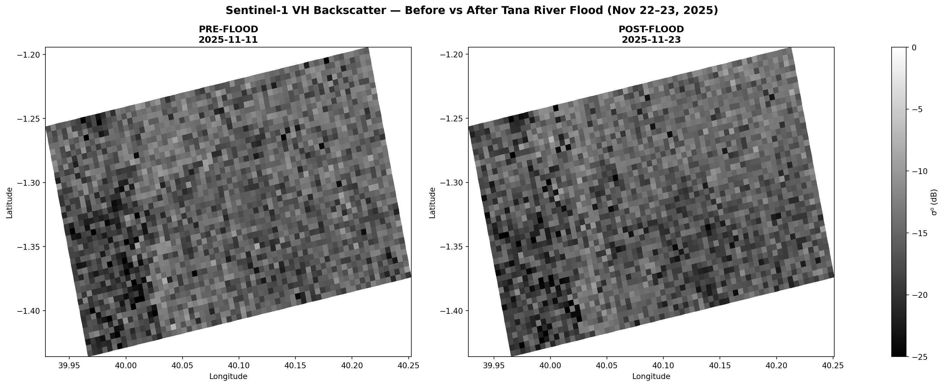
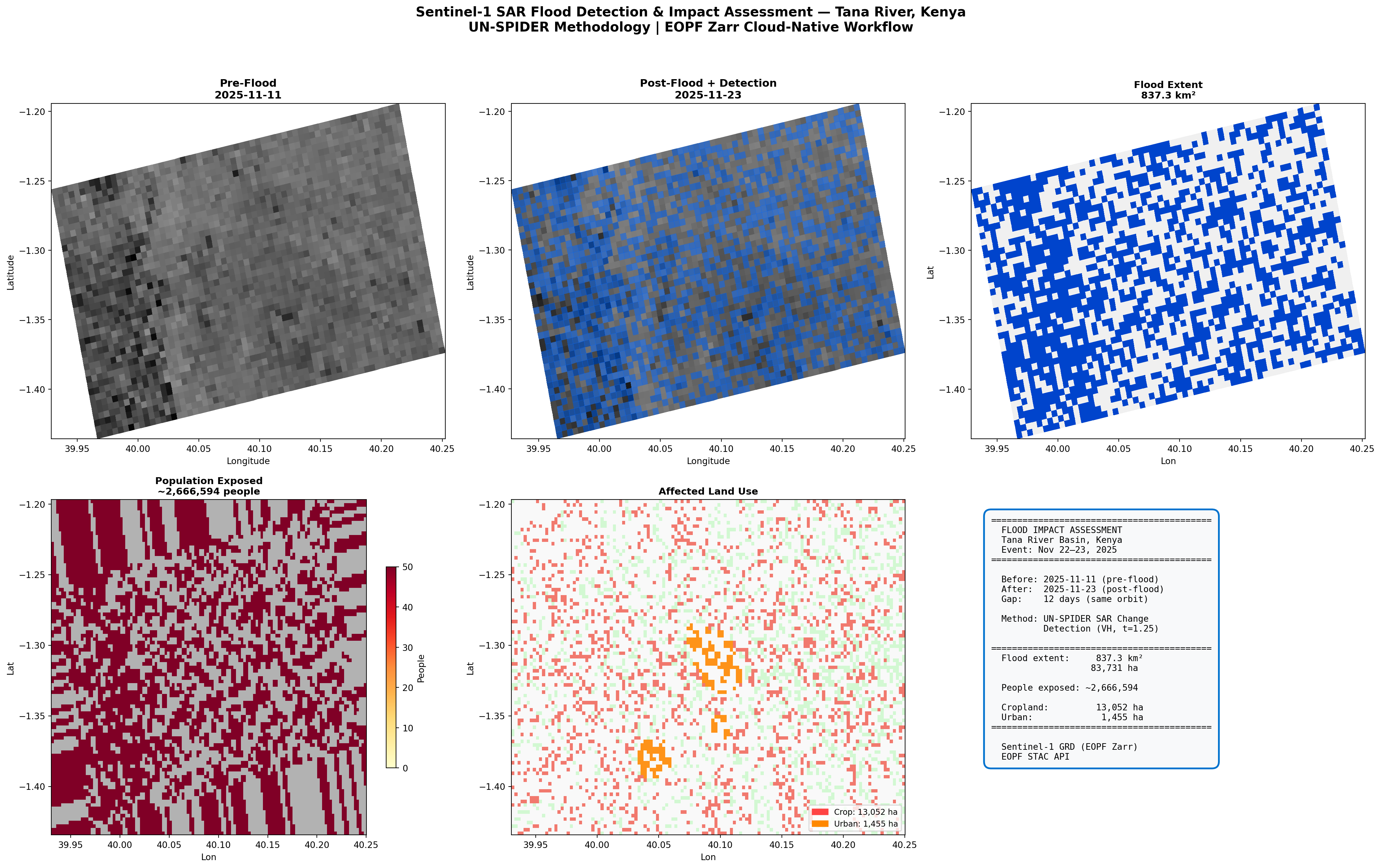
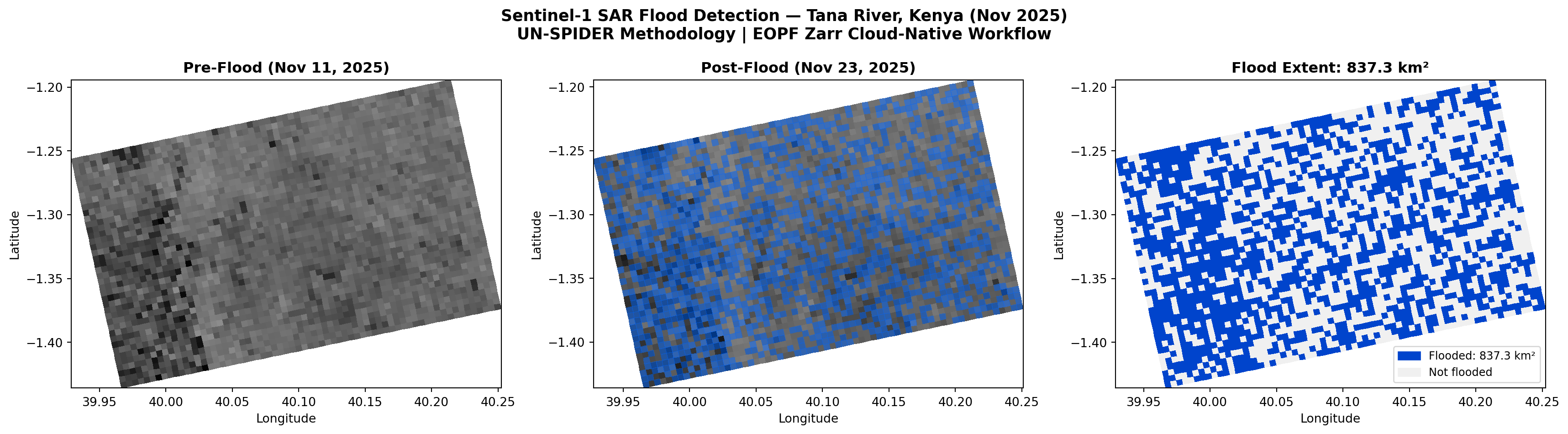
plot_sar(ax1, before_lon, before_lat, before_filt_db, s,
         f'Pre-Flood\n{before_item.datetime.strftime("%Y-%m-%d")}',
         valid_rows=bvr, valid_cols=bvc)

ax2 = fig.add_subplot(2, 3, 2)
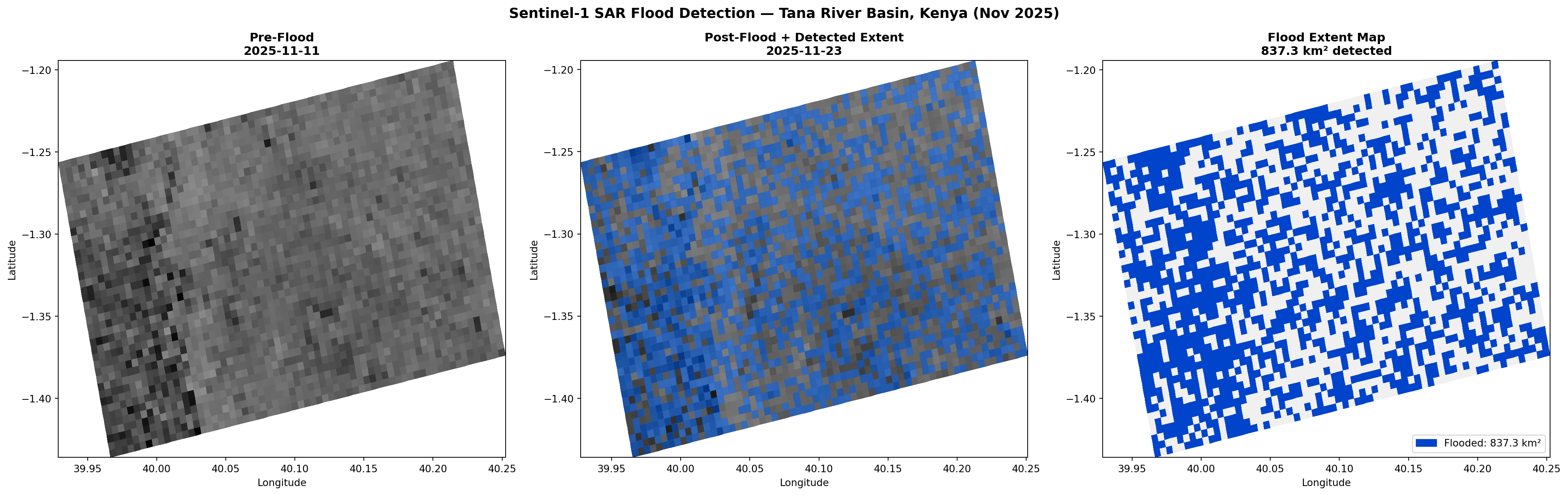
_, alon_c, alat_c = plot_sar(ax2, after_lon, after_lat, after_filt_db, s,
         f'Post-Flood + Detection\n{after_item.datetime.strftime("%Y-%m-%d")}',
         valid_rows=avr, valid_cols=avc)
fl_sub = subsample_to_coords(flood_refined, s, after_lat, avr, avc)
fl_ma = np.ma.masked_where(~fl_sub, fl_sub.astype(float))
ax2.pcolormesh(alon_c, alat_c, fl_ma, cmap=ListedColormap(['#0066FF']), alpha=0.5)

ax3 = fig.add_subplot(2, 3, 3)
fl_sub3 = subsample_to_coords(flood_refined, s, before_lat, bvr, bvc)
_, blon_c, blat_c = plot_sar(ax3, before_lon, before_lat, before_filt_db, s, '',
         valid_rows=bvr, valid_cols=bvc)
ax3.clear()
ax3.pcolormesh(blon_c, blat_c, fl_sub3.astype(int),
               cmap=ListedColormap(['#F0F0F0','#0044CC']), vmin=0, vmax=1)
ax3.set_title(f'Flood Extent\n{flood_km2:,.1f} kmΒ²', fontsize=11, fontweight='bold')
ax3.set_xlabel('Lon')
ax3.set_ylabel('Lat')

# Bottom row: Impact assessment
ax4 = fig.add_subplot(2, 3, 4)
ax4.pcolormesh(rlon, rlat, pop, cmap='Greys', vmin=0, vmax=100, alpha=0.3)
pe = np.ma.masked_where(~flood_reg, pop_exposed)
im4 = ax4.pcolormesh(rlon, rlat, pe, cmap='YlOrRd', vmin=0, vmax=50)
fig.colorbar(im4, ax=ax4, label='People', shrink=0.6)
ax4.set_title(f'Population Exposed\n~{total_exposed:,} people', fontsize=11, fontweight='bold')
ax4.set_xlabel('Lon')
ax4.set_ylabel('Lat')

ax5 = fig.add_subplot(2, 3, 5)
ax5.pcolormesh(rlon, rlat, ((lc==12)|(lc==14)).astype(float),
               cmap=ListedColormap(['#F0F0F0','#90EE90']), vmin=0, vmax=1, alpha=0.4)
ac = np.ma.masked_where(~crop_affected, crop_affected.astype(float))
ax5.pcolormesh(rlon, rlat, ac, cmap=ListedColormap(['#FF4444']), alpha=0.7)
au = np.ma.masked_where(~urban_affected, urban_affected.astype(float))
ax5.pcolormesh(rlon, rlat, au, cmap=ListedColormap(['#FF8800']), alpha=0.9)
ax5.legend(handles=[
    mpatches.Patch(color='#FF4444', label=f'Crop: {crop_ha:,} ha'),
    mpatches.Patch(color='#FF8800', label=f'Urban: {urban_ha:,} ha')
], loc='lower right', fontsize=9)
ax5.set_title('Affected Land Use', fontsize=11, fontweight='bold')
ax5.set_xlabel('Lon')
ax5.set_ylabel('Lat')

# Summary panel
ax6 = fig.add_subplot(2, 3, 6)
ax6.axis('off')
summary = (
    f"{'='*42}\n"
    f"  FLOOD IMPACT ASSESSMENT\n"
    f"  Tana River Basin, Kenya\n"
    f"  Event: Nov 22–23, 2025\n"
    f"{'='*42}\n\n"
    f"  Before: {before_item.datetime.strftime('%Y-%m-%d')} (pre-flood)\n"
    f"  After:  {after_item.datetime.strftime('%Y-%m-%d')} (post-flood)\n"
    f"  Gap:    12 days (same orbit)\n\n"
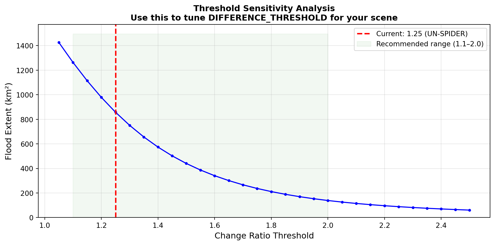
    f"  Method: UN-SPIDER SAR Change\n"
    f"          Detection (VH, t={effective_threshold})\n\n"
    f"{'='*42}\n"
    f"  Flood extent:  {flood_km2:>8,.1f} kmΒ²\n"
    f"                 {flood_ha:>8,.0f} ha\n\n"
    f"  People exposed: ~{total_exposed:>7,}\n\n"
    f"  Cropland:       {crop_ha:>8,} ha\n"
    f"  Urban:          {urban_ha:>8,} ha\n"
    f"{'='*42}\n\n"
    f"  Sentinel-1 GRD (EOPF Zarr)\n"
    f"  EOPF STAC API"
)
ax6.text(0.05, 0.95, summary, transform=ax6.transAxes, fontsize=10,
         fontfamily='monospace', va='top',
         bbox=dict(boxstyle='round,pad=0.8', fc='#f8f9fa', ec='#0072ce', lw=2))

fig.suptitle('Sentinel-1 SAR Flood Detection & Impact Assessment β€” Tana River, Kenya\n'
             'UN-SPIDER Methodology | EOPF Zarr Cloud-Native Workflow',
             fontsize=15, fontweight='bold', y=0.98)
plt.tight_layout(rect=[0,0,1,0.95])
plt.show()

πŸ“Έ Thumbnail

A compact summary image suitable for catalog listings and social sharing.

# Generate thumbnail image
fig_thumb, axes_t = plt.subplots(1, 3, figsize=(18, 5))
s = DISPLAY_STEP

# Pre-flood
plot_sar(axes_t[0], before_lon, before_lat, before_filt_db, s,
         f'Pre-Flood ({before_item.datetime.strftime("%b %d, %Y")})',
         valid_rows=bvr, valid_cols=bvc)

# Post-flood + flood overlay
_, alon_c, alat_c = plot_sar(axes_t[1], after_lon, after_lat, after_filt_db, s,
         f'Post-Flood ({after_item.datetime.strftime("%b %d, %Y")})',
         valid_rows=avr, valid_cols=avc)
fl_sub = subsample_to_coords(flood_refined, s, after_lat, avr, avc)
fl_ma = np.ma.masked_where(~fl_sub, fl_sub.astype(float))
axes_t[1].pcolormesh(alon_c, alat_c, fl_ma, cmap=ListedColormap(['#0066FF']), alpha=0.5)

# Clean flood map
fl_sub3 = subsample_to_coords(flood_refined, s, before_lat, bvr, bvc)
_, blon_c, blat_c = plot_sar(axes_t[2], before_lon, before_lat, before_filt_db, s, '',
         valid_rows=bvr, valid_cols=bvc)
axes_t[2].clear()
axes_t[2].pcolormesh(blon_c, blat_c, fl_sub3.astype(int),
                     cmap=ListedColormap(['#F0F0F0', '#0044CC']), vmin=0, vmax=1)
axes_t[2].set_title(f'Flood Extent: {flood_km2:,.1f} kmΒ²', fontsize=12, fontweight='bold')
axes_t[2].set_xlabel('Longitude')
axes_t[2].set_ylabel('Latitude')
flood_p = mpatches.Patch(color='#0044CC', label=f'Flooded: {flood_km2:,.1f} kmΒ²')
dry_p = mpatches.Patch(color='#F0F0F0', label='Not flooded')
axes_t[2].legend(handles=[flood_p, dry_p], loc='lower right', fontsize=9)

fig_thumb.suptitle('Sentinel-1 SAR Flood Detection β€” Tana River, Kenya (Nov 2025)\n'
                   'UN-SPIDER Methodology | EOPF Zarr Cloud-Native Workflow',
                   fontsize=13, fontweight='bold')
plt.tight_layout()
# fig_thumb.savefig('thumbnail.png', dpi=150, bbox_inches='tight', facecolor='white')
# print("Saved: thumbnail.png")
plt.show()

πŸ—ΊοΈ Interactive Flood Map

An interactive map lets you zoom, pan, and inspect the flood extent overlaid on satellite basemaps. This is critical for field teams who need to identify specific affected communities and access routes.

πŸ’‘ Tip: Use the layer control (top-right) to switch between OpenStreetMap and satellite imagery. Click the blue marker for a flood summary popup.

# Build interactive flood map with folium
center_lat = (before_lat.min() + before_lat.max()) / 2
center_lon = (before_lon.min() + before_lon.max()) / 2

m = folium.Map(location=[center_lat, center_lon], zoom_start=10,
               tiles='OpenStreetMap')

# Add satellite basemap layer
folium.TileLayer(
    tiles='https://server.arcgisonline.com/ArcGIS/rest/services/World_Imagery/MapServer/tile/{z}/{y}/{x}',
    attr='Esri', name='Satellite Imagery', overlay=False
).add_to(m)

# Subsample flood grid for performance
step_i = max(1, flood_reg.shape[0] // 150)
step_j = max(1, flood_reg.shape[1] // 150)
flood_small = flood_reg[::step_i, ::step_j]
lat_small = rlat[::step_i, ::step_j]
lon_small = rlon[::step_i, ::step_j]

# Add flood cells as rectangles
flood_group = folium.FeatureGroup(name='Flood Extent')
count = 0
cell_size = grid_res * step_i
for i in range(flood_small.shape[0]):
    for j in range(flood_small.shape[1]):
        if flood_small[i, j]:
            lat_i = float(lat_small[i, j])
            lon_j = float(lon_small[i, j])
            folium.Rectangle(
                bounds=[[lat_i, lon_j], [lat_i + cell_size, lon_j + cell_size]],
                color='#0044CC', fill=True, fill_color='#0066FF',
                fill_opacity=0.5, weight=0
            ).add_to(flood_group)
            count += 1
flood_group.add_to(m)

# Study area bounding box
folium.Rectangle(
    bounds=[[before_lat.min(), before_lon.min()],
            [before_lat.max(), before_lon.max()]],
    color='red', fill=False, weight=2,
    popup='Study Area'
).add_to(m)

# Info marker
flood_info = f"""<div style="font-size:12px; width:220px;">
<b>Tana River Flood</b><br>
Event: Nov 22-23, 2025<br>
Extent: {flood_km2:,.1f} km2<br>
People exposed: ~{total_exposed:,}<br>
Cropland: {crop_ha:,} ha<br>
<i>Sentinel-1 SAR / EOPF Zarr</i></div>"""
folium.Marker(
    location=[center_lat, center_lon],
    popup=folium.Popup(flood_info, max_width=250),
    icon=folium.Icon(color='blue', icon='info-sign')
).add_to(m)

folium.LayerControl().add_to(m)
print(f"Interactive map: {count} flood cells rendered")

# Display the map (works in all JupyterLab versions)
display(m)
Interactive map: 6200 flood cells rendered
Make this Notebook Trusted to load map: File -> Trust Notebook

πŸ’ͺ Now it is your turn

This workflow is designed to be reusable and adaptable. Try the challenges below!

Task 1: Change the Study Area 🌍

  • Visit bboxfinder.com and select a different flood-prone region (e.g., the Brahmaputra Delta, the Mekong, or the Mississippi)
  • Update BBOX and TARGET_LAT/TARGET_LON in the configuration cell
  • Search for matching Sentinel-1 image pairs and compare flood detection across different landscapes

Task 2: Tune the Detection Parameters πŸŽ›οΈ

  • Experiment with different DIFFERENCE_THRESHOLD values (1.1–2.0) and observe how flood extent changes
  • Try different SPECKLE_KERNEL sizes (5, 7, 15, 21) β€” smaller kernels preserve detail, larger ones reduce noise
  • Use the threshold sensitivity plot in Section 3.5 to find the optimal value for your study area

Task 3: Add Real Auxiliary Data πŸ“¦

  • Replace the synthetic population grid with GHSL GHS-POP data for validated exposure estimates
  • Integrate the JRC Global Surface Water layer to separate permanent water from new flooding
  • Add a DEM (e.g., SRTM) for slope masking to reduce false positives in hilly terrain

Task 4: Multi-temporal Flood Tracking πŸ“ˆ

  • Search for all available Sentinel-1 images across the full wet season (October–December 2025)
  • Generate a time series of flood extent maps to track flood progression and recession
  • Calculate the maximum flood extent and duration of inundation per pixel

Conclusion

This notebook demonstrated a complete SAR-based flood detection and impact assessment pipeline using Sentinel-1 Level-1 GRD data from the EOPF Zarr Sample Service.

What we accomplished:

Step Achievement
πŸ›°οΈ Cloud-native data access Discovered and loaded matched Sentinel-1 image pairs through the EOPF STAC API, reading only the spatial subset needed from remote Zarr stores instead of downloading 860 MB products
πŸ“‘ Full SAR processing chain Implemented radiometric calibration, GCP-based georeferencing, and speckle filtering to transform raw Digital Numbers into analysis-ready sigma nought backscatter
🌊 UN-SPIDER flood detection Applied ratio-based change detection with connected component refinement to map flood extent, capturing both open water and flooded vegetation
πŸ“Š Impact assessment Overlaid flood extent on population density and land cover to estimate affected populations, damaged cropland, and impacted urban areas

Key Insight #1
EOPF Zarr enables efficient, scalable processing β€” no bulk downloads needed

Key Insight #2
SAR works regardless of cloud cover β€” ideal for tropical flood events

Key Insight #3
Threshold requires iterative tuning per scene for optimal results

Limitations: - Terrain correction and slope masking (DEM) would reduce false positives in hilly areas - JRC Global Surface Water masking would separate permanent water bodies from new flooding - Real population/land cover datasets would provide validated impact numbers


What’s next?

This workflow opens the door to operational flood monitoring with EOPF data:

πŸ“¦ Real Auxiliary Datasets
Integrate GHSL GHS-POP, WorldPop, and MODIS land cover for validated impact assessment

πŸ“ˆ Multi-temporal Tracking
Process all available images across the wet season to map flood progression and recession dynamics

πŸ”„ Cross-sensor Validation
Combine with Sentinel-2 optical data (also in EOPF Zarr) during cloud-free windows for independent verification

⚑ Automated Alerting
Deploy as a near-real-time monitoring system using the EOPF STAC API to trigger analysis when new S1 acquisitions arrive

In the next notebook, we will explore a workflow for vegetation productivity and drought monitoring in the Horn of Africa, with EOPF Zarr data from the EOPF STAC Catalog

This notebook was developed as a contribution to the EOPF Zarr Community Notebook Competition.