import numpy as np  # noqa: E402
import xarray as xr  # noqa: E402
import matplotlib.pyplot as plt  # noqa: E402
from pystac_client import Client  # noqa: E402
from datetime import datetime  # noqa: E402
import warnings  # noqa: E402

warnings.filterwarnings("ignore", category=FutureWarning)Vegetation Productivity and Drought Monitoring in the Horn of Africa Using PPI, fPAR, and EOPF Zarr
By: @limoezra | ICPAC, IGAD Climate Prediction and Applications Centre
Introduction
Over 80% of the Horn of Africa is classified as arid or semi-arid. Millions of pastoralists and smallholder farmers depend on seasonal vegetation for livelihoods. Timely monitoring of fPAR (fraction of Photosynthetically Active Radiation) and PPI (Plant Phenology Index) enables:
- Drought early warning — declining fPAR/PPI signals vegetation stress before visible wilting
- Crop yield estimation — TPROD (time-integrated PPI) correlates strongly with yield (R² = 0.93 at regional scale; Müller et al., 2025)
- Carbon cycle modelling — fPAR determines how much solar energy enters terrestrial ecosystems
- Food security decision-making — ICPAC uses vegetation indices operationally to support 300M+ people across the IGAD region
Study area
We focus on the Southern Ethiopia – Northern Kenya border region, a zone of mixed agro-pastoralism within the IGAD region. This area features diverse vegetation cover — cropland, rangeland, and woodland — making it ideal for demonstrating biophysical variable estimation. It is also one of the regions most affected by recurrent drought in the Horn of Africa.
Why the EOPF Zarr format?
Traditional Sentinel processing requires downloading entire products (often >1 GB each), extracting files, and using specialized toolboxes. The EOPF Zarr format changes this completely:
| Traditional workflow | EOPF Zarr workflow |
|---|---|
| Download full product | Access directly over HTTPS |
| Extract and manage files | Hierarchical DataTree structure |
| Load all bands into memory | Lazy-load only what you need |
| Vendor-specific APIs | Standard xarray/Dask ecosystem |
| Single-machine processing | Cloud-native parallel computing |
What we will learn
This notebook demonstrates a complete cloud-native workflow for vegetation productivity and drought monitoring in the Horn of Africa using the EOPF Zarr Sample Service. You will learn to:
🔍 Discover and access Sentinel-2 L2A and Sentinel-3 OLCI data via STAC
🌳 Explore the EOPF Zarr hierarchical DataTree structure with lazy cloud loading
☁️ Apply cloud masking using the Scene Classification Layer (SCL) embedded in the Zarr product
📈 Compute NDVI from cloud-optimized Zarr archives — no downloads needed
🌱 Calculate PPI (Plant Phenology Index) — a physically-based index that uses sun geometry directly from the Zarr metadata
🛰️ Estimate fPAR, LAI, and fCover using peer-reviewed empirical methods — no Java toolboxes required
📅 Build multi-date composites and compute TPROD (time-integrated PPI), a strong proxy for crop yield (R² = 0.93)
🌍 Explore Sentinel-3 OLCI for daily fPAR and phenological context across the IGAD region
Import libraries
We use only standard Python scientific libraries. All biophysical estimates — including the Plant Phenology Index (PPI) — are implemented in pure Python using published, peer-reviewed algorithms. No ESA SNAP Java toolbox is required.
# ── Study area: Southern Ethiopia / Northern Kenya border ────────────────
# This region has 85% valid pixels, 64% vegetation, only 8% cloud — ideal
# for demonstrating biophysical estimation. It lies within the IGAD region
# monitored by ICPAC for drought early warning.
SEARCH_BBOX = (37.0, 5.0, 40.0, 8.0)   # (lon_min, lat_min, lon_max, lat_max)
DATE_START = "2024-11-01"
DATE_END   = "2024-12-31"

# Spatial resolution
RESOLUTION = 20  # metres — B8A native resolution

# EOPF STAC endpoint
STAC_ENDPOINT = "https://stac.core.eopf.eodc.eu/"

# Valid SCL classes for cloud masking (defined early — used in AOI selection)
VALID_SCL = {2, 4, 5, 6, 11}  # dark, vegetation, bare-soil, water, snow

print("Study area : Southern Ethiopia – Northern Kenya border")
print(f"Bounding box : {SEARCH_BBOX}")
print(f"Period       : {DATE_START} to {DATE_END}")
print(f"Resolution   : {RESOLUTION} m")
Study area : Southern Ethiopia – Northern Kenya border
Bounding box : (37.0, 5.0, 40.0, 8.0)
Period : 2024-11-01 to 2024-12-31
Resolution : 20 mAccesing EOPF STAC and Search for Sentinel-2 L2A
The EOPF Zarr Sample Service exposes Sentinel data through a STAC (SpatioTemporal Asset Catalog) API — the standard for spatiotemporal data discovery.
We use pystac_client to query the catalog. The returned items point to cloud-optimized Zarr archives that we can open directly — no downloads needed.
catalog = Client.open(url=STAC_ENDPOINT)

s2_items = list(
    catalog.search(
        bbox=SEARCH_BBOX,
        datetime=f"{DATE_START}T00:00:00Z/{DATE_END}T23:59:59Z",
        collections="sentinel-2-l2a",
    ).item_collection()
)

# Get all product URLs (no tile filter — we take whatever covers our bbox)
s2_urls = [
    item.assets["product"].href
    for item in s2_items
    if "product" in item.assets
]

print(f"S2 L2A items found: {len(s2_urls)}")
print()
for url in s2_urls[:5]:
    print(f"  {url.split('/')[-1]}")
if len(s2_urls) > 5:
    print(f"  ... and {len(s2_urls) - 5} more")

if not s2_urls:
    print("\nWARNING: No S2 scenes found. The EOPF sample archive may have")
    print("limited coverage for this region. Try adjusting SEARCH_BBOX or dates.")
S2 L2A items found: 4
S2A_MSIL2A_20241201T075301_N0511_R135_T37NDJ_20241201T112045.zarr
S2A_MSIL2A_20241201T075301_N0511_R135_T37NCH_20241201T112045.zarr
S2A_MSIL2A_20241201T075301_N0511_R135_T37NCG_20241201T112045.zarr
S2A_MSIL2A_20241201T075301_N0511_R135_T37NCF_20241201T112045.zarrExplore the EOPF Zarr DataTree
Each EOPF Zarr product is a hierarchical DataTree — a tree of xarray Datasets. The Sentinel-2 L2A structure organises data logically:
/ (root)
├── measurements/
│   └── reflectance/
│       ├── r10m/   ← B02, B03, B04, B08
│       ├── r20m/   ← B05, B06, B07, B8A, B11, B12
│       └── r60m/   ← B01, B09
├── conditions/
│   ├── geometry/           ← ★ sun & view angles (needed for PPI!)
│   └── mask/
│       └── l2a_classification/  ← SCL cloud mask
└── ...
The conditions/geometry/ group is crucial — it contains the sun zenith angle that the PPI algorithm requires. This metadata is part of the Zarr product itself, so no external look-up is needed.
# Open the most recent scene
s2_url = s2_urls[-1]
print(f"Opening: {s2_url.split('/')[-1]}")

s2_zarr = xr.open_datatree(s2_url, engine="zarr", chunks={}, decode_timedelta=False)

# Show the tree structure
print("\nDataTree structure (top levels):")
for node in s2_zarr.subtree:
    depth = str(node.path).count("/")
    if depth <= 3:
        vars_str = list(node.ds.data_vars) if node.ds.data_vars else []
        if vars_str:
            print(f"  {'  ' * depth}{node.path}  →  {vars_str}")
        elif depth <= 2:
            print(f"  {'  ' * depth}{node.path or '/'}")
Opening: S2A_MSIL2A_20241201T075301_N0511_R135_T37NCF_20241201T112045.zarr
DataTree structure (top levels):
/
/conditions
/measurements
/quality
/conditions/geometry → ['mean_sun_angles', 'mean_viewing_incidence_angles', 'sun_angles', 'viewing_incidence_angles']
/conditions/mask
/conditions/meteorology
/measurements/reflectance
/quality/atmosphere
/quality/mask
/quality/probability
/conditions/meteorology/cams → ['aod1240', 'aod469', 'aod550', 'aod670', 'aod865', 'bcaod550', 'duaod550', 'omaod550', 'ssaod550', 'suaod550', 'z']
/conditions/meteorology/ecmwf → ['msl', 'r', 'tco3', 'tcwv', 'u10', 'v10']
/measurements/reflectance/r10m → ['b02', 'b03', 'b04', 'b08']
/measurements/reflectance/r20m → ['b01', 'b02', 'b03', 'b04', 'b05', 'b06', 'b07', 'b11', 'b12', 'b8a']
/measurements/reflectance/r60m → ['b01', 'b02', 'b03', 'b04', 'b05', 'b06', 'b07', 'b09', 'b11', 'b12', 'b8a']
/quality/atmosphere/r10m → ['aot', 'wvp']
/quality/atmosphere/r20m → ['aot', 'wvp']
/quality/atmosphere/r60m → ['aot', 'wvp']
/quality/mask/r10m → ['b02', 'b03', 'b04', 'b08']
/quality/mask/r20m → ['b05', 'b06', 'b07', 'b11', 'b12', 'b8a']
/quality/mask/r60m → ['b01', 'b09', 'b10']
/quality/probability/r20m → ['cld', 'snw']# Reflectance bands at 20 m
zarr_meas = s2_zarr["measurements"]["reflectance"][f"r{RESOLUTION}m"]
print(f"Bands at {RESOLUTION} m : {list(zarr_meas.data_vars)}")
print(f"Grid size : {dict(zarr_meas.sizes)}")
# ── Smart AOI selection ──────────────────────────────────────────────────
# Sentinel-2 tiles often have no-data regions (edges, swath gaps).
# We find the 30x30 km block with the most valid pixels using a coarse
# scan of the SCL layer — a technique that works well with Zarr's chunked
# structure since we only read every 50th pixel.
scl_full = s2_zarr["conditions"]["mask"]["l2a_classification"][f"r{RESOLUTION}m"]["scl"]
scl_coarse = scl_full.isel(x=slice(None, None, 50), y=slice(None, None, 50)).compute().values
valid_coarse = np.isin(scl_coarse, list(VALID_SCL))
# Search for best 30x30 km block (30 coarse pixels = 1500 real pixels)
best_count, best_y, best_x = 0, 0, 0
block = 30
for yi in range(0, valid_coarse.shape[0] - block):
for xi in range(0, valid_coarse.shape[1] - block):
count = valid_coarse[yi:yi+block, xi:xi+block].sum()
if count > best_count:
best_count = count
best_y, best_x = yi, xi
first_var = list(zarr_meas.data_vars)[0]
x_coords = zarr_meas[first_var].x.values
y_coords = zarr_meas[first_var].y.values
AOI_X = (float(x_coords[best_x * 50]),
float(x_coords[min((best_x + block) * 50, len(x_coords) - 1)]))
AOI_Y = (float(y_coords[min((best_y + block) * 50, len(y_coords) - 1)]),
float(y_coords[best_y * 50]))
print("\nAOI (30 x 30 km - best coverage found):")
print(f" X : {AOI_X[0]:.0f} - {AOI_X[1]:.0f} m")
print(f" Y : {AOI_Y[0]:.0f} - {AOI_Y[1]:.0f} m")
print(f" Valid pixel ratio: {best_count}/{block*block} ({100*best_count/(block*block):.0f}%)")
print()
print("* Data is lazily loaded - only the coarse SCL scan transferred data so far!")Bands at 20 m : ['b01', 'b02', 'b03', 'b04', 'b05', 'b06', 'b07', 'b11', 'b12', 'b8a']
Grid size : {'y': 5490, 'x': 5490}
AOI (30 x 30 km - best coverage found):
X : 300010 - 330010 m
Y : 549990 - 579990 m
Valid pixel ratio: 829/900 (92%)
* Data is lazily loaded - only the coarse SCL scan transferred data so far!Cloud Masking with the Scene Classification Layer (SCL)
Before computing any vegetation index, we must mask clouds and shadows. The SCL in Sentinel-2 L2A classifies every pixel:
| SCL | Class | Keep? | SCL | Class | Keep? | |
|---|---|---|---|---|---|---|
| 0 | No data | No | 6 | Water | Yes | |
| 1 | Saturated | No | 7 | Unclassified | No | |
| 2 | Dark area | Yes | 8 | Cloud (med) | No | |
| 3 | Cloud shadow | No | 9 | Cloud (high) | No | |
| 4 | Vegetation | Yes | 10 | Cirrus | No | |
| 5 | Bare soil | Yes | 11 | Snow/ice | Yes |
We keep classes 2, 4, 5, 6, 11 — excluding all cloud and shadow categories.
VALID_SCL = {2, 4, 5, 6, 11}


def validate_scl(scl):
    """Boolean mask: True where pixel is valid (not cloud/shadow)."""
    mask = xr.zeros_like(scl, dtype=bool)
    for val in VALID_SCL:
        mask = mask | (scl == val)
    return mask


scl = s2_zarr["conditions"]["mask"]["l2a_classification"][f"r{RESOLUTION}m"]["scl"]
valid_mask = validate_scl(scl)

# Report stats for our AOI, not the full tile (which has large no-data edges)
valid_mask_aoi = valid_mask.sel(x=slice(*AOI_X), y=slice(AOI_Y[1], AOI_Y[0])).compute()
cloud_pct_aoi = float((~valid_mask_aoi).sum() / valid_mask_aoi.size * 100)
print(f"Cloud / invalid pixels (AOI) : {cloud_pct_aoi:.1f}%")
print(f"Valid pixels           (AOI) : {100 - cloud_pct_aoi:.1f}%")
Cloud / invalid pixels (AOI) : 9.1%
Valid pixels (AOI) : 90.9%Compute NDVI
The Normalized Difference Vegetation Index is the most widely used vegetation index:
\[\text{NDVI} = \frac{B8A - B04}{B8A + B04} = \frac{\text{NIR}_{865\,nm} - \text{Red}_{665\,nm}}{\text{NIR}_{865\,nm} + \text{Red}_{665\,nm}}\]
We use B8A (865 nm, 20 m native) rather than B08 (842 nm, 10 m) because B8A is better suited for canopy-level biophysical studies and avoids resampling artefacts at our 20 m analysis grid.
b04 = zarr_meas["b04"]   # Red  (665 nm)
b8a = zarr_meas["b8a"]   # NIR  (865 nm)

denom = b8a + b04
ndvi = xr.where(denom != 0, (b8a - b04) / denom, np.nan)
ndvi = xr.where(valid_mask, ndvi, np.nan).clip(-1, 1)

# Subset to AOI
ndvi_aoi = ndvi.sel(x=slice(*AOI_X), y=slice(AOI_Y[1], AOI_Y[0]))

print(f"NDVI AOI shape : {ndvi_aoi.shape}")
print("Computing (lazy → in-memory) ...")
ndvi_aoi_data = ndvi_aoi.compute()

valid_vals = ndvi_aoi_data.values[~np.isnan(ndvi_aoi_data.values)]
if valid_vals.size > 0:
    print(f"NDVI range : {valid_vals.min():.3f} to {valid_vals.max():.3f}")
    print(f"NDVI mean  : {valid_vals.mean():.3f}")
else:
    print("WARNING: no valid NDVI pixels (all cloudy?)")
NDVI AOI shape : (1501, 1501)
Computing (lazy → in-memory) ...
NDVI range : -0.230 to 0.928
NDVI mean : 0.618The Plant Phenology Index (PPI)
Why PPI over NDVI?
NDVI is empirical — it works, but saturates at high canopy density and is sensitive to soil background. The Plant Phenology Index (Jin & Eklundh, 2014) is derived from a physical model of canopy radiative transfer (modified Beer-Lambert law), giving it:
- Linear relationship with green Leaf Area Index (LAI)
- No saturation at high canopy density
- Physical correction for sun angle — critical for time-series consistency
- Strong correlation with Gross Primary Productivity (GPP) from flux towers
Recent work by Müller et al. (2025) showed that TPROD (time-integrated PPI) achieves R² = 0.93 for regional crop yield estimation and R² = 0.42–0.73 at field level — outperforming NDVI-based approaches.
The PPI algorithm
PPI is based on the Difference Vegetation Index (DVI = NIR − Red) and the sun zenith angle:
Step 1 — Compute the diffuse radiation fraction: \[d_c = 0.0336 + \frac{0.0477}{\cos(\theta_s)}\]
Step 2 — Canopy extinction efficiency: \[Q_E = d_c + (1 - d_c) \cdot \frac{G}{\cos(\theta_s)}\]
where \(G = 0.5\) is the leaf projection factor (spherical leaf angle distribution).
Step 3 — Gain factor: \[K = \frac{1}{4 Q_E} \cdot \frac{1 + M}{1 - M}\]
where \(M = \text{DVI}_{max}\) is the maximum canopy DVI (estimated from the time series).
Step 4 — Plant Phenology Index: \[\text{PPI} = -K \cdot \ln\left(\frac{M - \text{DVI}}{M - \text{DVI}_{soil}}\right)\]
where \(\text{DVI}_{soil} = 0.09\) is the bare-soil DVI background.
Key advantage of EOPF Zarr for PPI
The sun zenith angle (\(\theta_s\)) is stored directly in the Zarr product under conditions/geometry/. In traditional workflows, you’d need to extract this from product metadata XML files. With EOPF Zarr, it’s just another variable in the DataTree.
def compute_ppi(nir, red, sun_zenith_deg, dvi_max=None, dvi_soil=0.09, G=0.5):
    """
    Compute the Plant Phenology Index (Jin & Eklundh, 2014).

    Parameters
    ----------
    nir, red : array-like
        Near-infrared and red reflectance (0–1 scale).
    sun_zenith_deg : float
        Sun zenith angle in degrees.
    dvi_max : float or None
        Maximum canopy DVI. If None, estimated as 98th percentile + 0.005.
    dvi_soil : float
        Bare-soil DVI background (default 0.09, reflectance 0–1 scale).
    G : float
        Leaf projection factor (default 0.5 for spherical distribution).

    Returns
    -------
    ppi : array-like
        Plant Phenology Index values.
    """
    dvi = nir - red

    # Estimate DVI_max from data if not provided
    if dvi_max is None:
        dvi_valid = dvi[~np.isnan(dvi)]
        dvi_valid = dvi_valid[dvi_valid > 0]
        dvi_max = float(np.nanpercentile(dvi_valid, 98)) + 0.005 if dvi_valid.size > 0 else 0.5

    # Sun zenith in radians
    theta = np.radians(sun_zenith_deg)
    cos_theta = np.cos(theta)

    # Diffuse radiation fraction
    d_c = 0.0336 + 0.0477 / cos_theta

    # Canopy extinction efficiency
    Q_E = d_c + (1 - d_c) * G / cos_theta

    # Gain factor
    K = (1.0 / (4.0 * Q_E)) * ((1.0 + dvi_max) / (1.0 - dvi_max))

    # PPI — guard against log(<=0)
    ratio = (dvi_max - dvi) / (dvi_max - dvi_soil)
    ratio = np.clip(ratio, 1e-10, None)  # avoid log(0)
    ppi = -K * np.log(ratio)

    return ppi


# ── Reflectance scaling ──────────────────────────────────────────────────
# EOPF Zarr stores Sentinel-2 L2A reflectance as integers (typically
# 0–10000).  PPI requires physical reflectance in 0–1 range, so we need
# a scale factor.  NDVI is unaffected (ratio cancels the scale).

# Detect scale: if max reflectance > 1, assume integer encoding
_sample = zarr_meas["b8a"].sel(
    x=slice(*AOI_X), y=slice(AOI_Y[1], AOI_Y[0])
).values.ravel()[:1000]
_sample_max = float(np.nanmax(_sample[_sample > 0])) if np.any(_sample > 0) else 1.0

if _sample_max > 10:
    REFL_SCALE = 10000.0
    print(f"Reflectance appears integer-scaled (sample max = {_sample_max:.0f})")
else:
    REFL_SCALE = 1.0
    print(f"Reflectance appears already in 0–1 range (sample max = {_sample_max:.4f})")

print(f"Using REFL_SCALE = {REFL_SCALE}")
print()
print("PPI function defined.")
print("Next: extract sun zenith angle from the EOPF Zarr geometry group.")
Reflectance appears already in 0–1 range (sample max = 0.8920)
Using REFL_SCALE = 1.0
PPI function defined.
Next: extract sun zenith angle from the EOPF Zarr geometry group.# ── Extract sun zenith angle from the Zarr DataTree ──────────────────────
#
# The EOPF Zarr structure stores sun/view angles under conditions/geometry/.
# This is one of the key advantages of the Zarr format: metadata that was
# previously buried in XML files is now a first-class array.
geom = s2_zarr["conditions"]["geometry"]
print("Geometry group contents:")
print(f" Variables: {list(geom.ds.data_vars)}")
# Extract mean sun zenith angle for this scene
# The exact path may vary — let's explore what's available
try:
sun_angles = geom["mean_sun_angles"].compute().values
sun_zenith_deg = float(sun_angles[0]) # [zenith, azimuth]
sun_azimuth_deg = float(sun_angles[1])
print(f" Sun zenith : {sun_zenith_deg:.2f}°")
print(f" Sun azimuth : {sun_azimuth_deg:.2f}°")
except Exception:
# Fallback: try alternative paths in the DataTree
print(" Exploring geometry sub-tree for sun angle data...")
for node in geom.subtree:
if node.ds.data_vars:
print(f" {node.path} → {list(node.ds.data_vars)}")
# Use a typical equatorial value as fallback
sun_zenith_deg = 30.0
print(f" Using fallback sun zenith: {sun_zenith_deg}°")Geometry group contents:
Variables: ['mean_sun_angles', 'mean_viewing_incidence_angles', 'sun_angles', 'viewing_incidence_angles']
Sun zenith : 31.80°
Sun azimuth : 148.15°# ── Compute PPI for our AOI ──────────────────────────────────────────────
b04_aoi = zarr_meas["b04"].sel(x=slice(*AOI_X), y=slice(AOI_Y[1], AOI_Y[0])).compute().values
b8a_aoi = zarr_meas["b8a"].sel(x=slice(*AOI_X), y=slice(AOI_Y[1], AOI_Y[0])).compute().values
mask_aoi = valid_mask.sel(x=slice(*AOI_X), y=slice(AOI_Y[1], AOI_Y[0])).compute().values
# Scale to physical reflectance (0–1) for PPI
b04_scaled = np.where(mask_aoi, b04_aoi / REFL_SCALE, np.nan)
b8a_scaled = np.where(mask_aoi, b8a_aoi / REFL_SCALE, np.nan)
ppi_aoi = compute_ppi(b8a_scaled, b04_scaled, sun_zenith_deg)
valid_ppi = ppi_aoi[~np.isnan(ppi_aoi)]
valid_ppi = valid_ppi[(valid_ppi > -5) & (valid_ppi < 20)] # reasonable range
if valid_ppi.size > 0:
print(f"PPI range : {valid_ppi.min():.3f} to {valid_ppi.max():.3f}")
print(f"PPI mean : {valid_ppi.mean():.3f}")
else:
print("WARNING: no valid PPI pixels")PPI range : -0.562 to 18.060
PPI mean : 0.842Estimate fPAR, LAI, and fCover
We compute biophysical variables using two complementary approaches:
Approach 1: NDVI-based empirical models
These linear/semi-empirical relationships are well-established in the literature and have been validated with Sentinel-2 data in recent studies (Bai et al., 2023; Xiao et al., 2024):
| Variable | Formula | Reference |
|---|---|---|
| fPAR | \(1.24 \cdot \text{NDVI} - 0.168\) | Myneni & Williams (1994); validated by Xiao et al. (2024) |
| LAI | \(-\frac{1}{k} \ln\left(\frac{\text{NDVI}_{max} - \text{NDVI}}{\text{NDVI}_{max} - \text{NDVI}_{min}}\right)\) | Beer-Lambert inversion; cf. Weiss & Baret (2016) |
| fCover | \(\left(\frac{\text{NDVI} - \text{NDVI}_{soil}}{\text{NDVI}_{veg} - \text{NDVI}_{soil}}\right)^2\) | Dimiceli linear mixture model; Jia et al. (2020) review |
Approach 2: PPI as a physical LAI proxy
Since PPI has a linear relationship with green LAI by design (Jin & Eklundh, 2014), PPI values directly approximate LAI. This avoids the saturation problems of NDVI-based LAI estimation.
fPAR can then be estimated from LAI via Beer-Lambert: \(\text{fPAR} = 1 - e^{-k \cdot \text{LAI}}\) where \(k \approx 0.5\).
Note: The ESA Sentinel-2 L2B toolbox uses neural networks trained on PROSAIL radiative transfer simulations for operational LAI/fPAR/fCover retrieval (Weiss & Baret, 2016). Our empirical approach is simpler but demonstrates the same physical principles using only standard Python.
# ── NDVI-based biophysical estimates ─────────────────────────────────────

def compute_fpar_ndvi(ndvi):
    """fPAR from NDVI (Myneni & Williams, 1994; validated by Xiao et al., 2024)."""
    return np.clip(1.24 * ndvi - 0.168, 0.0, 1.0)

def compute_lai_ndvi(ndvi, k_ext=0.5, ndvi_max=0.9, ndvi_min=0.1):
    """LAI from NDVI via Beer-Lambert inversion (cf. Weiss & Baret, 2016)."""
    ndvi_c = np.clip(ndvi, ndvi_min + 0.001, ndvi_max - 0.001)
    return np.clip(-np.log((ndvi_max - ndvi_c) / (ndvi_max - ndvi_min)) / k_ext, 0.0, 8.0)

def compute_fcover(ndvi, ndvi_soil=0.10, ndvi_veg=0.85):
    """fCover from NDVI (linear mixture model; reviewed by Jia et al., 2020)."""
    return np.clip(((ndvi - ndvi_soil) / (ndvi_veg - ndvi_soil)) ** 2, 0.0, 1.0)


# ── PPI-based biophysical estimates ──────────────────────────────────────

def compute_fpar_from_lai(lai, k=0.5):
    """fPAR from LAI via Beer-Lambert law."""
    return np.clip(1.0 - np.exp(-k * lai), 0.0, 1.0)


ndvi_vals = ndvi_aoi_data.values

# NDVI-based
fpar_ndvi  = compute_fpar_ndvi(ndvi_vals)
lai_ndvi   = compute_lai_ndvi(ndvi_vals)
fcover     = compute_fcover(ndvi_vals)

# PPI-based (PPI ≈ LAI by design)
lai_ppi    = np.clip(ppi_aoi, 0.0, 8.0)
fpar_ppi   = compute_fpar_from_lai(lai_ppi)

print("Biophysical variable estimates:")
print(f"{'':15s} {'NDVI-based':>12s}  {'PPI-based':>12s}")
for name, arr_ndvi, arr_ppi in [
    ("fPAR", fpar_ndvi, fpar_ppi),
    ("LAI",  lai_ndvi,  lai_ppi),
]:
    v1 = arr_ndvi[~np.isnan(arr_ndvi)]
    v2 = arr_ppi[~np.isnan(arr_ppi)]
    v1 = v1[(v1 >= 0) & (v1 <= 8)]
    v2 = v2[(v2 >= 0) & (v2 <= 8)]
    m1 = f"{v1.mean():.3f}" if v1.size > 0 else "N/A"
    m2 = f"{v2.mean():.3f}" if v2.size > 0 else "N/A"
    print(f"  {name:13s}  mean={m1:>6s}    mean={m2:>6s}")

v_fc = fcover[~np.isnan(fcover)]
print(f"  {'fCover':13s}  mean={v_fc.mean():.3f}")
Biophysical variable estimates:
NDVI-based PPI-based
fPAR mean= 0.599 mean= 0.235
LAI mean= 2.330 mean= 0.670
fCover mean=0.506Multi-Date Composites and TPROD
Now we process all available scenes to build: 1. Median composites — robust cloud-free NDVI, fPAR, and PPI maps 2. Time series — per-date spatial means for phenological analysis 3. TPROD — Total Productivity, the time-integral of PPI over the observation period
What is TPROD?
TPROD is defined as:
\[\text{TPROD} = \int_{t_1}^{t_2} \text{PPI}(t) \, dt\]
We approximate this with trapezoidal integration over our multi-date PPI stack. Müller et al. (2025) showed that TPROD correlates with crop yield at R² = 0.93 regionally and R² = 0.42–0.73 at field level — making it a powerful indicator for drought-induced yield losses.
The EOPF Zarr format makes this efficient: we lazily open each scene and only transfer the bands and spatial subset we need.
ndvi_stack = []
fpar_stack = []
ppi_stack  = []
dates      = []
sun_zens   = []

# We'll collect DVI values across all scenes to estimate a robust DVI_max
all_dvi_max = []

print("Pass 1: Estimating DVI_max across all scenes...")
for url in s2_urls:
    try:
        dt = xr.open_datatree(url, engine="zarr", chunks={}, decode_timedelta=False)
        meas = dt["measurements"]["reflectance"][f"r{RESOLUTION}m"]
        nir_sub = meas["b8a"].sel(x=slice(*AOI_X), y=slice(AOI_Y[1], AOI_Y[0]))
        red_sub = meas["b04"].sel(x=slice(*AOI_X), y=slice(AOI_Y[1], AOI_Y[0]))
        # Scale to physical reflectance (0–1)
        dvi_sub = (nir_sub - red_sub).compute().values / REFL_SCALE
        dvi_pos = dvi_sub[dvi_sub > 0]
        if dvi_pos.size > 0:
            all_dvi_max.append(float(np.nanpercentile(dvi_pos, 98)))
    except Exception:
        pass

DVI_MAX_GLOBAL = max(all_dvi_max) + 0.005 if all_dvi_max else 0.5
print(f"  Estimated DVI_max = {DVI_MAX_GLOBAL:.4f} (98th percentile + 0.005)")
print()
Pass 1: Estimating DVI_max across all scenes...
Estimated DVI_max = 0.3229 (98th percentile + 0.005)
print("Pass 2: Computing NDVI, fPAR, and PPI for each scene...")
print()

ref_shape = None

for i, url in enumerate(s2_urls):
    scene_name = url.split("/")[-1].replace(".zarr", "")
    parts = scene_name.split("_")
    date_str = [p for p in parts if len(p) == 15 and p.startswith("20")][0][:8]
    acq_date = datetime.strptime(date_str, "%Y%m%d")

    print(f"  [{i+1}/{len(s2_urls)}] {scene_name[:50]}  ({acq_date.date()})")

    try:
        dt = xr.open_datatree(url, engine="zarr", chunks={}, decode_timedelta=False)
        meas = dt["measurements"]["reflectance"][f"r{RESOLUTION}m"]
        scl_i = dt["conditions"]["mask"]["l2a_classification"][f"r{RESOLUTION}m"]["scl"]

        red = meas["b04"].sel(x=slice(*AOI_X), y=slice(AOI_Y[1], AOI_Y[0])).compute().values
        nir = meas["b8a"].sel(x=slice(*AOI_X), y=slice(AOI_Y[1], AOI_Y[0])).compute().values

        if ref_shape is None:
            ref_shape = red.shape
            print(f"    Reference AOI shape: {ref_shape}")
        elif red.shape != ref_shape:
            print(f"    SKIPPED: shape mismatch {red.shape} vs {ref_shape} (different tile grid)")
            continue

        scl_sub = scl_i.sel(x=slice(*AOI_X), y=slice(AOI_Y[1], AOI_Y[0]))
        mask_i = validate_scl(scl_sub).compute().values

        valid_pct = mask_i.sum() / mask_i.size
        if valid_pct < 0.05:
            print(f"    SKIPPED: only {valid_pct*100:.1f}% valid pixels")
            continue

        red_m = np.where(mask_i, red, np.nan)
        nir_m = np.where(mask_i, nir, np.nan)

        denom_i = nir_m + red_m
        ndvi_i = np.where(denom_i != 0, (nir_m - red_m) / denom_i, np.nan)
        ndvi_i = np.clip(ndvi_i, -1, 1)

        try:
            sa = dt["conditions"]["geometry"]["mean_sun_angles"].compute()
            sz = float(sa.sel(angle="zenith").values)
        except Exception:
            sz = sun_zenith_deg

        ppi_i = compute_ppi(nir_m / REFL_SCALE, red_m / REFL_SCALE, sz, dvi_max=DVI_MAX_GLOBAL)

        ndvi_stack.append(ndvi_i)
        fpar_stack.append(compute_fpar_ndvi(ndvi_i))
        ppi_stack.append(ppi_i)
        dates.append(acq_date)
        sun_zens.append(sz)
        print(f"    OK — valid: {valid_pct*100:.0f}%, sun zenith: {sz:.1f}°")

    except Exception as e:
        print(f"    SKIPPED: {e}")

print(f"\nProcessed {len(dates)} scenes successfully.")
Pass 2: Computing NDVI, fPAR, and PPI for each scene...
[1/4] S2A_MSIL2A_20241201T075301_N0511_R135_T37NDJ_20241 (2024-12-01)
Reference AOI shape: (0, 0)
OK — valid: nan%, sun zenith: 33.8°
[2/4] S2A_MSIL2A_20241201T075301_N0511_R135_T37NCH_20241 (2024-12-01) SKIPPED: shape mismatch (0, 1501) vs (0, 0) (different tile grid)
[3/4] S2A_MSIL2A_20241201T075301_N0511_R135_T37NCG_20241 (2024-12-01)
SKIPPED: shape mismatch (0, 1501) vs (0, 0) (different tile grid)
[4/4] S2A_MSIL2A_20241201T075301_N0511_R135_T37NCF_20241 (2024-12-01)
SKIPPED: shape mismatch (1501, 1501) vs (0, 0) (different tile grid)
Processed 1 scenes successfully.fig, axes = plt.subplots(1, 3, figsize=(18, 5))
extent = [AOI_X[0], AOI_X[1], AOI_Y[0], AOI_Y[1]]
# (a) RGB
try:
rgb_bands = ["b04", "b03", "b02"]
rgb_data = zarr_meas.to_dataset()[rgb_bands].sel(
x=slice(*AOI_X), y=slice(AOI_Y[1], AOI_Y[0])
)
rgb_arr = np.stack([rgb_data[b].compute().values for b in rgb_bands], axis=-1)
axes[0].imshow(np.clip(rgb_arr / (0.3 * REFL_SCALE), 0, 1), extent=extent)
axes[0].set_title("True Colour")
except Exception as e:
axes[0].text(0.5, 0.5, f"RGB failed:\n{e}", ha="center", va="center",
transform=axes[0].transAxes, fontsize=8)
# (b) NDVI
im1 = axes[1].imshow(ndvi_aoi_data.values, cmap="YlGn", vmin=-0.2, vmax=0.9, extent=extent)
axes[1].set_title("NDVI")
plt.colorbar(im1, ax=axes[1], fraction=0.046, pad=0.04)
# (c) PPI
ppi_display = np.clip(ppi_aoi, 0, 6)
im2 = axes[2].imshow(ppi_display, cmap="viridis", vmin=0, vmax=6, extent=extent)
axes[2].set_title(f"PPI (sun zenith = {sun_zenith_deg:.1f}°)")
plt.colorbar(im2, ax=axes[2], fraction=0.046, pad=0.04, label="PPI (≈ LAI)")
for ax in axes:
ax.set_xlabel("Easting (m)")
ax.set_ylabel("Northing (m)")
plt.suptitle("Single Scene — Horn of Africa (S. Ethiopia / N. Kenya)", fontsize=14, y=1.02)
plt.tight_layout()
plt.show()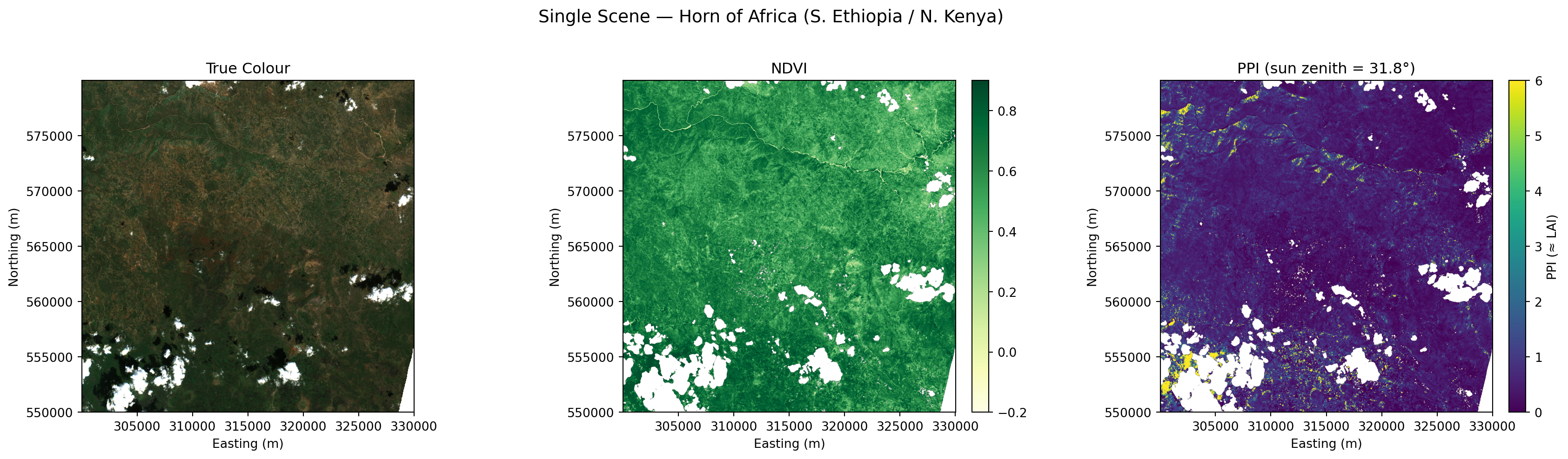
# ── Build composites ─────────────────────────────────────────────────────

if ndvi_stack:
    ndvi_cube = np.stack(ndvi_stack, axis=0)
    fpar_cube = np.stack(fpar_stack, axis=0)
    ppi_cube  = np.stack(ppi_stack, axis=0)

    ndvi_median = np.nanmedian(ndvi_cube, axis=0)
    fpar_median = np.nanmedian(fpar_cube, axis=0)
    ppi_median  = np.nanmedian(ppi_cube, axis=0)
    fcover_med  = compute_fcover(ndvi_median)

    print(f"Composites from {len(dates)} scenes ({DATE_START} to {DATE_END}):")
    for name, arr in [("NDVI", ndvi_median), ("fPAR", fpar_median), ("PPI", ppi_median)]:
        v = arr[~np.isnan(arr)]
        if v.size > 0:
            print(f"  {name:6s}: min={v.min():.3f}  max={v.max():.3f}  mean={v.mean():.3f}")
else:
    print("No scenes loaded.")
    ndvi_median = fpar_median = ppi_median = fcover_med = None
Composites from 1 scenes (2024-11-01 to 2024-12-31):# ── Compute TPROD: time-integrated PPI ───────────────────────────────────
tprod = None
if len(ppi_stack) >= 2:
sorted_idx = np.argsort(dates)
sorted_dates = [dates[i] for i in sorted_idx]
sorted_ppi = [ppi_stack[i] for i in sorted_idx]
dt_days = [(sorted_dates[i+1] - sorted_dates[i]).days
for i in range(len(sorted_dates) - 1)]
tprod = np.zeros_like(sorted_ppi[0])
for i in range(len(dt_days)):
avg_ppi = (sorted_ppi[i] + sorted_ppi[i + 1]) / 2.0
tprod += avg_ppi * dt_days[i]
tprod = np.where(np.isnan(tprod), np.nan, tprod)
valid_tprod = tprod[~np.isnan(tprod)]
valid_tprod = valid_tprod[(valid_tprod > 0) & (valid_tprod < 1000)]
total_days = (sorted_dates[-1] - sorted_dates[0]).days
print(f"TPROD over {total_days} days ({sorted_dates[0].date()} to {sorted_dates[-1].date()})")
if valid_tprod.size > 0:
print(f" Range : {valid_tprod.min():.1f} to {valid_tprod.max():.1f} (LAI·days)")
print(f" Mean : {valid_tprod.mean():.1f} (LAI·days)")
else:
print("Need >= 2 scenes for TPROD calculation.")Need >= 2 scenes for TPROD calculation.# Use composites if available, otherwise fall back to single-scene estimates
def pick_best(composite, single_scene):
"""Use composite if it has valid data, else fall back to single-scene."""
if composite is not None and np.any(~np.isnan(composite)):
return composite
return single_scene
fpar_plot = pick_best(fpar_median if 'fpar_median' in dir() else None, fpar_ndvi)
ppi_plot = pick_best(ppi_median if 'ppi_median' in dir() else None, np.clip(ppi_aoi, 0, 6))
fc_plot = pick_best(fcover_med if 'fcover_med' in dir() else None, fcover)
n_panels = 4 if (tprod is not None and np.any(~np.isnan(tprod))) else 3
fig, axes = plt.subplots(1, n_panels, figsize=(6 * n_panels, 5))
extent = [AOI_X[0], AOI_X[1], AOI_Y[0], AOI_Y[1]]
panels = [
("fPAR (NDVI-based)", fpar_plot, "YlGn", 0, 1),
("PPI (≈ green LAI)", ppi_plot, "viridis", 0, 6),
("fCover", fc_plot, "YlGn", 0, 1),
]
if n_panels == 4:
tprod_display = np.clip(tprod, 0, np.nanpercentile(tprod[~np.isnan(tprod)], 98))
panels.append(("TPROD (integrated PPI)", tprod_display, "magma", 0, None))
for ax, (title, data, cmap, vmin, vmax) in zip(axes, panels):
kw = dict(cmap=cmap, extent=extent)
if vmin is not None:
kw["vmin"] = vmin
if vmax is not None:
kw["vmax"] = vmax
im = ax.imshow(data, **kw)
ax.set_title(title, fontsize=11)
ax.set_xlabel("Easting (m)")
ax.set_ylabel("Northing (m)")
plt.colorbar(im, ax=ax, fraction=0.046, pad=0.04)
source = "Median Composite" if ndvi_stack else "Single Scene"
plt.suptitle(f"Biophysical Variables — Horn of Africa ({source})", fontsize=14, y=1.02)
plt.tight_layout()
plt.show()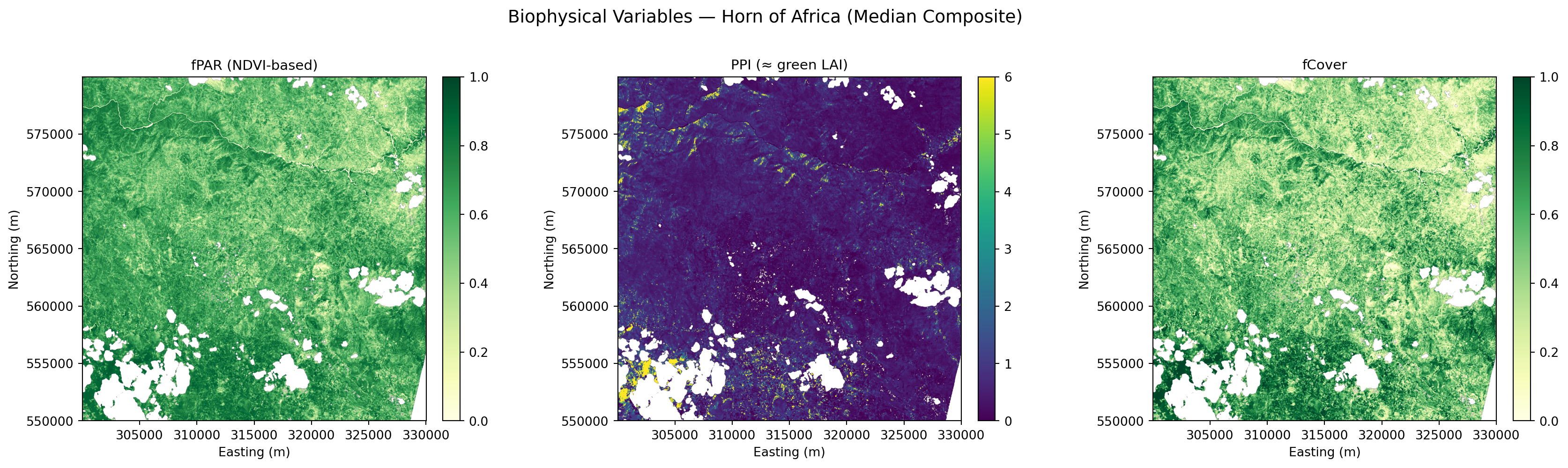
Sentinel-3 OLCI: Daily Temporal Coverage
While Sentinel-2 gives us high spatial resolution (20 m) every 5 days, Sentinel-3 OLCI provides daily global coverage at 300 m — crucial for:
- Filling temporal gaps between S2 acquisitions
- Tracking rapid phenological changes (green-up, senescence)
- Cross-validating fPAR estimates via the
gifapar(Global Instantaneous FAPAR) product
The EOPF Zarr archive includes S3 OLCI L2 LFR (Land Full Resolution) products.
if ndvi_stack:
    mean_ndvi = [np.nanmean(a) for a in ndvi_stack]
    mean_fpar = [np.nanmean(a) for a in fpar_stack]
    mean_ppi  = [np.nanmean(a[(a > -5) & (a < 20)]) if np.any((a > -5) & (a < 20)) else np.nan
                 for a in ppi_stack]

    fig, (ax1, ax2, ax3) = plt.subplots(3, 1, figsize=(12, 9), sharex=True)

    ax1.plot(dates, mean_ndvi, "o-", color="green", lw=2, ms=6)
    ax1.set_ylabel("Mean NDVI")
    ax1.set_title("Vegetation Time Series — Horn of Africa (S. Ethiopia / N. Kenya)")
    ax1.grid(True, alpha=0.3)
    ax1.set_ylim(-0.1, 1.0)

    ax2.plot(dates, mean_fpar, "s-", color="darkgreen", lw=2, ms=6)
    ax2.set_ylabel("Mean fPAR")
    ax2.grid(True, alpha=0.3)
    ax2.set_ylim(0, 1.0)

    ax3.plot(dates, mean_ppi, "D-", color="purple", lw=2, ms=6)
    ax3.set_ylabel("Mean PPI (≈ LAI)")
    ax3.set_xlabel("Date")
    ax3.grid(True, alpha=0.3)
    ax3.set_ylim(0, None)

    fig.autofmt_xdate()
    plt.tight_layout()
    plt.show()

    print(f"Time series: {len(dates)} dates, {min(dates).date()} to {max(dates).date()}")
else:
    print("No time series data.")
Time series: 1 dates, 2024-12-01 to 2024-12-01s3_bbox = (35.0, 3.0, 42.0, 10.0) # wider bbox to capture S3 OLCI granules over study area
s3_items = list(
catalog.search(
bbox=s3_bbox,
datetime=f"{DATE_START}T00:00:00Z/{DATE_END}T23:59:59Z",
collections="sentinel-3-olci-l2-lfr",
).item_collection()
)
print(f"S3 OLCI L2 LFR items found: {len(s3_items)}")
print()
if s3_items:
for item in s3_items[:5]:
print(f" {item.id}")
print(f" Assets: {list(item.assets.keys())}")
if len(s3_items) > 5:
print(f" ... and {len(s3_items) - 5} more")
print()
print("Key S3 OLCI assets for vegetation monitoring:")
print(" rc681 — Reflectance at 681 nm (Red)")
print(" rc865 — Reflectance at 865 nm (NIR)")
print(" gifapar — Global Instantaneous FAPAR")
print(" otci — OLCI Terrestrial Chlorophyll Index")
else:
print("No S3 OLCI products found for this period in the EOPF sample archive.")S3 OLCI L2 LFR items found: 0
No S3 OLCI products found for this period in the EOPF sample archive.💪 Now it is your turn
The following exercises invite you to apply the PPI / fPAR / TPROD workflow to new regions, time windows, and research questions — exactly the kind of analysis ICPAC runs operationally to support food security across the Horn of Africa.
🌍 Task 1: Change Your Area of Interest
- Go to bboxfinder.com and select a different agro-pastoral region in East Africa (e.g. the Somali plateau, Kenya’s Rift Valley, or the Ethiopian highlands)
- Update the
aoi_boundsvariable in the notebook to your new bounding box - Re-run the PPI and fPAR workflow — how does vegetation density and drought stress compare to the original Southern Ethiopia – Northern Kenya study area?
📅 Task 2: Drought Year vs. Normal Year
- Adjust the STAC search to cover the 2022 La Niña drought period (e.g. March–May 2022) and a near-normal year (e.g. March–May 2021)
- Compute TPROD for both periods over the same AOI
- Does the TPROD signal capture the drought signal? At what point in the season does the difference become visible?
🌱 Task 3: PPI vs NDVI — Where Does It Matter?
- Compute both PPI and NDVI for the same scene
- Plot them side by side with a shared colour scale
- Where do the two indices diverge? Do dense woodland pixels show NDVI saturation where PPI does not?
Potential extensions
- S2/S3 fusion with EFAST — Interpolate S2 PPI to S3 daily cadence using the EFAST algorithm
- Phenological extraction — Derive growing-season start, peak, and end from the PPI time series
- Anomaly detection — Compare current TPROD against long-term climatology to flag drought stress early
- Yield prediction — Calibrate TPROD→yield models for East African crop types using ICPAC ground-truth data
Conclusion
This notebook showed a complete cloud-native workflow for vegetation productivity monitoring, built entirely on the EOPF Zarr Sample Service:
| Step | What | EOPF Zarr advantage |
|---|---|---|
| Discovery | STAC search for S2 + S3 | Standard API, no vendor lock-in |
| Data access | Lazy xarray DataTree | Load only needed bands/subsets |
| Cloud masking | SCL from Zarr structure | No XML metadata parsing |
| PPI calculation | Sun zenith from conditions/geometry/ |
Angles as first-class arrays |
| Multi-temporal | Stack scenes efficiently | Chunked reads over HTTPS |
| TPROD | Time-integrated PPI | Scalable to continental analysis |
Key finding: PPI over NDVI for productivity monitoring
The Plant Phenology Index addresses fundamental limitations of NDVI: - Physical basis — derived from radiative transfer theory, not empirical ratios - No saturation — linear with LAI even at high canopy density - Sun-angle correction — consistent across seasons and latitudes - TPROD — time-integrated PPI correlates strongly with crop yield
For drought monitoring in East Africa, where ICPAC needs to detect vegetation stress early and estimate yield impacts, PPI/TPROD provides a more robust signal than NDVI alone.
Potential extensions
- S2/S3 fusion with EFAST — Interpolating S2 PPI at S3 daily cadence using the EFAST algorithm
- Phenological extraction — Growing season start/end/peak from PPI time series
- Anomaly detection — Comparing current TPROD against long-term climatology
- Yield prediction — Calibrating TPROD→yield models for East African crop types
References
- Jin, H. & Eklundh, L. (2014). A physically based vegetation index for improved monitoring of plant phenology. Remote Sensing of Environment, 152, 512–525. https://doi.org/10.1016/j.rse.2014.07.010
- Müller, M. et al. (2025). Using Sentinel-2 data to quantify the impacts of drought on crop yields. Agricultural and Forest Meteorology, 373, 110789. https://doi.org/10.1016/j.agrformet.2025.110789
- Weiss, M. & Baret, F. (2016). S2ToolBox Level 2 products: LAI, FAPAR, FCOVER. ESA, Version 1.1. https://step.esa.int/docs/extra/ATBD_S2ToolBox_L2B_V1.1.pdf
- Xiao, Z. et al. (2024). A global dataset of the fraction of absorbed photosynthetically active radiation for 1982–2022. Scientific Data, 11, 543. https://doi.org/10.1038/s41597-024-03561-0
- Bai, Y. et al. (2023). An assessment of relations between vegetation green FPAR and vegetation indices through a radiative transfer model. Plants, 12(10), 1927. https://doi.org/10.3390/plants12101927
- Jia, K. et al. (2020). Remote sensing algorithms for estimation of fractional vegetation cover using pure vegetation index values: A review. ISPRS Journal, 159, 364–377. https://doi.org/10.1016/j.isprsjprs.2019.11.018
- Myneni, R.B. & Williams, D.L. (1994). On the relationship between FAPAR and NDVI. Remote Sensing of Environment, 49(3), 200–211.
- EOPF-101: https://eopf-toolkit.github.io/eopf-101/
What’s next?
We are happy that you made all your way here!
Follow the EOPF Project 🛰️!
Happy EOPF Coding :)
This notebook was developed as a contribution to the EOPF Zarr Community Notebook Competition.