An introduction to Chunking
Introduction
Chunking is the secret sauce that makes .zarr format incredibly efficient for Earth Observation data processing.
Understanding chunking allows us to transform the way we work with massive satellite datasets. This means somehow, turning memory-crushing, slow operations into fast, scalable analysis workflows.
This introduction takes you from chunking basics to advanced optimisation strategies specifically tailored for EOPF (Earth Observation Processing Framework) datasets.
What we will learn
- 🧱 What a chunk is
- ⏳ Recognise the relationship between chunk and optimisation
- 📚 The relevant considerations for chunking size, compression and transfer
What are chunks?
Zarr revolutionises how we store and access large multidimensional arrays by breaking them into smaller, manageable pieces called chunks. Think of chunks as rectangular tiles that together compose a complete dataset, but with a significant difference: they allow us to access and process each of the components independently.
A chunk is .zarr’s fundamental storage unit: an equally-sized block of array data that gets compressed and stored as a separate object.
For example, when we have a massive 10,000 × 10,000 pixel satellite image, zarr might divide it into 100 chunks of 1,000 × 1,000 pixels each. Then, each chunk becomes a separate compressed file or object in our storage system.
Why chunks transform performance
Chunking addresses three critical performance bottlenecks in large-scale data processing:
Memory efficiency: Instead of loading entire datasets into RAM, chunks allow us to only load the specific data we need. This allows us to work with datasets larger than our available memory, like a 100 GB satellite time series. It can be processed on a machine with just 8 GB of RAM.
I/O optimisation: Chunking minimises data transfer, as it only reads relevant sections. When we need data from one geographic region,
zarrloads only those chunks covering that area. For cloud storage, this translates to fewer, more efficient HTTP requests instead of downloading massive files. It also reduces data latency.Parallel processing: Different chunks can be processed simultaneously by multiple CPU cores or distributed workers. This transforms compute-intensive operations from sequential bottlenecks into scalable parallel workflows.
Chunk sizes for performance
Chunk size selection fundamentally determines the performance characteristics over our dataset. The choice of chunking size affects memory usage, I/O efficiency, parallel scaling, and network transfer costs. That is the reason, it is one of the most critical optimisation decisions in Earth Observation data processing.
There are three levels of chunk sizes:
| Chunk size | Advantages | Disadvantages |
|---|---|---|
| Small chunks (1-10 MB) | Fine-grained access patterns, minimise memory usage per operation, and enable high granularity for parallel processing. | High metadata overhead, requires numerous network requests for cloud storage, and creates complex task graphs. |
| Medium chunks (10-100 MB) | Optimal balance for most Earth Observation applications, works well with cloud storage byte-range requests, enables efficient compression ratios, and supports good parallelisation without excessive overhead. | Depend exclusively on the dataset size, making it difficult to replicate |
| Large chunks (>100 MB) | Maximises compression efficiency, minimises network request count, and dramatically reduces metadata overhead for massive datasets. | Increases memory requirements, may transfer unnecessary data for sparse access patterns, and can limit parallel efficiency. |
A simple chunking example
We can explore chunking with a simple 2D raster dataset example. Imagine we have a 6×6 grid representing temperature data. This simple dataset can be chunked in different ways, each with its own advantages and tradeoffs:
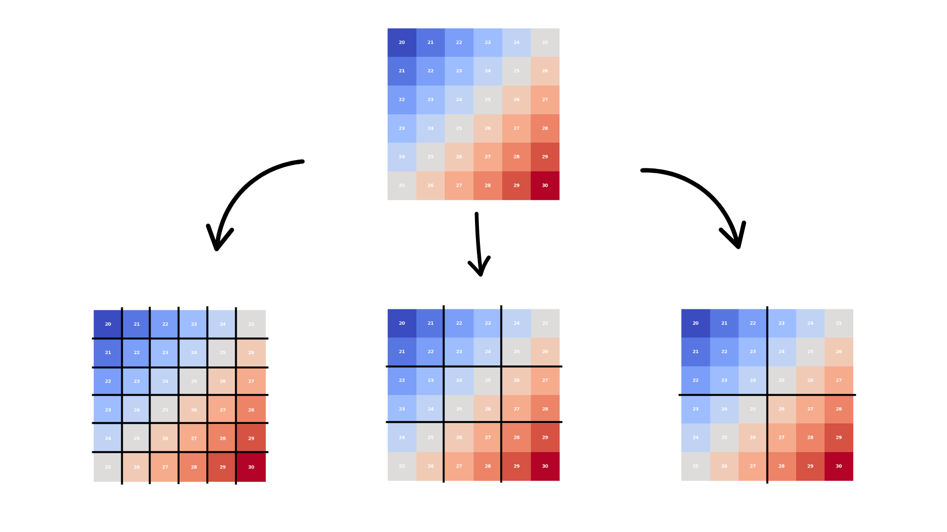
| 1×1 Chunks | 2×2 Chunks | 3×3 Chunks |
|---|---|---|
| - Each pixel is a chunk - Maximum flexibility but high overhead - 36 total chunks - Good for random access to individual cells - Poor for operations that need adjacent cells |
- Each chunk contains 4 cells - Balanced approach - 9 total chunks - Good for small region operations - Reasonable compression potential |
- Each chunk contains 9 cells - More efficient storage - 4 total chunks - Better compression - Less granular access |
Compression of chunks
Compression interactions significantly affect optimal chunk sizes. Larger chunks generally achieve better compression ratios, which are important for spectral data with high spatial correlation. However, compressed chunks must be fully decompressed when accessed, potentially increasing memory usage beyond the nominal chunk size. Balance compression benefits with memory requirements for your specific workflows.
The available compression algorithms for zarr are the following.
| Compression Algorithm | Description |
|---|---|
| Blosc with LZ4 | Provides excellent speed with moderate compression ratios, making it ideal for interactive applications where decompression speed matters more than maximum storage efficiency. LZ4 typically achieves 2-5× compression on satellite data with very fast decompression. |
| Zstandard (Zstd) | Offers an exceptional balance between compression ratio and speed, making it the preferred choice for many Earth Observation applications. Zstd often achieves 3-8× compression on spectral data while maintaining reasonable decompression performance. |
| Specialised algorithms | Such as JPEG 2000, provide excellent compression for certain data types but may not integrate well with general-purpose array processing workflows. Consider format compatibility when selecting compression approaches. |
Compression effectiveness depends heavily on network characteristics:
Bandwidth-limited environments benefit tremendously from aggressive compression since decompression is typically faster than network transfer. In these cases, higher compression ratios directly translate to reduced analysis time.
High-bandwidth, low-latency networks may make compression counterproductive if decompression becomes the bottleneck. Profile your specific network environment to determine optimal compression levels.
Cloud storage considerations include both transfer costs and access speed. Compressed data reduces both storage costs and transfer times, but increases CPU usage. For most Earth Observation applications, compression provides net benefits.
Why is it relevant to chunk EO data
Earth Observation datasets exhibit characteristics that significantly influence optimal chunking strategies. We can consider their structure, sizes, processing workflows and spatial and temporal resolutions.
Multi-dimensional complexity: Satellite data combines spatial dimensions (often tens of thousands of pixels per side), spectral dimensions (multiple wavelength bands), and temporal dimensions (time series spanning years or decades). Each dimension has different access patterns and computational requirements.
Scale characteristics: Modern satellites generate massive data volumes. The Sentinel-2 mission alone, for example, produces approximately 1.6 TB per orbit, with the full archive exceeding 25 petabytes and growing rapidly. Processing workflows must handle this scale efficiently.
Access patterns: Unlike general-purpose arrays, EO data has predictable access patterns. Spatial analysis typically accesses rectangular geographic regions. Spectral analysis needs multiple bands for the same locations. Time series analysis follows individual pixels or regions through time.
Heterogeneous resolutions: Many instruments capture data at multiple spatial resolutions simultaneously. Some missions require coordinated chunking strategies that balance storage efficiency with processing convenience.
💪 Now it is your turn
For a deep dive into the chunking theory and further technical resources, we recommend going through the following resources:
- Chunks and Chunkability: Tyranny of the Chunk
- Choosing Good Chunk Sizes in Dask - Dask team’s chunking recommendations
- Optimization Practices - Chunking - ESIP Fed’s chunking best practices
- Optimal Chunking Strategies for Cloud-based Storage - Research on geospatial chunking
Conclusion
This chapter introduced the logic behind data chunking and its relevance for scalable analysis workflows. We explored how optimising the size, compression and considering the transfer of these chunks significantly enhances the efficiency of data retrieval.
What’s next?
In the following section , we will go over optimal chunking strategies and relevant considerations when aiming for making Earth Observation workflows more efficient.