Access the EOPF Zarr STAC API with R

Introduction

In this section, we will explore programmatic access of the EOPF Zarr Collections available in the EOPF Sentinel Zarr Sample Service STAC Catalog using R. We will introduce R packages that enable us to effectively access and search through STAC catalogs.

What we will learn

• 🔍 How to programmatically browse through available collections available via the EOPF Zarr STAC Catalog, using the rstac package.
• 📊 Explore collection metadata in user-friendly terms
• 🎯 How to search for specific data

Prerequisites

An R environment is required to follow this tutorial, with R version >= 4.4.0. For local development, we recommend using either RStudio or Positron and making use of RStudio projects for a self-contained coding environment.

The rstac package is required to follow this tutorial. You can install it directly from CRAN:

install.packages("rstac")

Then load the package into your environment:

library(rstac)

Connect to the EOPF Sample Service STAC API

To access the EOPF Sample Service STAC catalog in R, we need to give the URL of the STAC API source (https://stac.core.eopf.eodc.eu/) using the function stac().

The object stac_source is a query containing information used to connect to the API, but it does not actually make any requests. To make requests to the API, we will always need to use get_request() or put_request(), as appropriate. Running get_request() on stac_source actually retrieves the catalogue:

stac_source <- stac("https://stac.core.eopf.eodc.eu/")

stac_source |>
  get_request()

## ###Catalog
## - id: eopf-sample-service-stac-api
## - description: STAC catalog of the EOPF Sentinel Zarr Samples Service
## - field(s): type, id, title, description, stac_version, conformsTo, links, stac_extensions

Browse collections

A STAC Collection exists to relate similar data sets together through space, time, and shared metadata. Each Sentinel mission and the downstream analysis-ready data are examples of STAC Collections. To browse STAC Collections, the collections() function is used. We can see that there are 11 collections available in the API:

stac_collections <- stac_source |>
  collections() |>
  get_request()

stac_collections

## ###Collections
## - collections (11 item(s)):
##   - sentinel-2-l2a
##   - sentinel-3-olci-l2-lfr
##   - sentinel-1-l2-ocn
##   - sentinel-3-slstr-l2-lst
##   - sentinel-1-l1-grd
##   - sentinel-2-l1c
##   - sentinel-1-l1-slc
##   - sentinel-3-slstr-l1-rbt
##   - sentinel-3-olci-l1-efr
##   - sentinel-3-olci-l1-err
##   - sentinel-3-olci-l2-lrr
## - field(s): collections, links, numberMatched, numberReturned

The default printing of the stac_collections() object summarises what’s been returned, but does not give all of the information. To see more about what’s been returned, we use str().

stac_collections |>
  str(max.level = 1)

## List of 4
##  $ collections   :List of 11
##  $ links         :List of 3
##   ..- attr(*, "class")= chr [1:2] "doc_links" "list"
##  $ numberMatched : int 11
##  $ numberReturned: int 11
##  - attr(*, "class")= chr [1:3] "doc_collections" "rstac_doc" "list"

Here, we can see that there is an entry "collections" within stac_collections, which we access to return the collections themselves (using head() to only return a few). This shows additional details about each collection, such as the collection id, title, description, and additional fields in the collections.

stac_collections[["collections"]] |>
  head(3)

## [[1]]
## ###Collection
## - id: sentinel-2-l2a
## - title: Sentinel-2 Level-2A
## - description: 
## The Sentinel-2 Level-2A Collection 1 product provides orthorectified Surface Reflectance (Bottom-Of-Atmosphere: BOA), with sub-pixel multispectral and multitemporal registration accuracy. Scene Classification (including Clouds and Cloud Shadows), AOT (Aerosol Optical Thickness) and WV (Water Vapour) maps are included in the product.
## - field(s): 
## id, type, links, title, assets, extent, license, keywords, providers, summaries, description, item_assets, stac_version, stac_extensions
## 
## [[2]]
## ###Collection
## - id: sentinel-3-olci-l2-lfr
## - title: Sentinel-3 OLCI Level-2 LFR
## - description: 
## The Sentinel-3 OLCI L2 LFR product provides land and atmospheric geophysical parameters computed for full resolution.
## - field(s): 
## id, type, links, title, assets, extent, license, keywords, providers, summaries, description, item_assets, stac_version, stac_extensions
## 
## [[3]]
## ###Collection
## - id: sentinel-1-l2-ocn
## - title: Sentinel-1 Level-2 OCN
## - description: 
## The Sentinel-1 Level-2 Ocean (OCN) products for wind, wave and currents applications may contain the following geophysical components derived from the SAR data: Ocean Wind field (OWI), Ocean Swell spectra (OSW), Surface Radial Velocity (RVL). The availability of components depends on the acquisition mode. The metadata referring to OWI are derived from an internally processed GRD product, the metadata referring to RVL (and OSW, for SM and WV mode) are derived from an internally processed SLC product.
## - field(s): 
## id, type, links, title, assets, extent, license, keywords, providers, summaries, description, item_assets, stac_version, stac_extensions

The Sentinel-2 Level-2A collection can be accessed by getting the first entry in stac_collections()[["collections"]]

stac_collections[["collections"]][[1]]

## ###Collection
## - id: sentinel-2-l2a
## - title: Sentinel-2 Level-2A
## - description: 
## The Sentinel-2 Level-2A Collection 1 product provides orthorectified Surface Reflectance (Bottom-Of-Atmosphere: BOA), with sub-pixel multispectral and multitemporal registration accuracy. Scene Classification (including Clouds and Cloud Shadows), AOT (Aerosol Optical Thickness) and WV (Water Vapour) maps are included in the product.
## - field(s): 
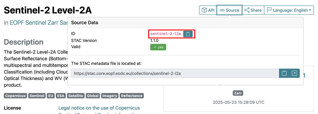
## id, type, links, title, assets, extent, license, keywords, providers, summaries, description, item_assets, stac_version, stac_extensions

However, the best way to access a specific collection is to search for it directly using the collection ID. The ID, “sentinel-2-l2a”, is visible in the Collection output above. It is also accessible in the browsable STAC catalog of the EOPF Sentinel Zarr Samples Service, on the page for that collection, under “Source.”

The collection ID can be supplied directly in the collections() function. If we look at the query without getting the result, we can see that it has been formed using the collection_id, “sentinel-2-l2a”, as a filter parameter.

sentinel_2_l2a_query <- stac_source |>
  collections(collection_id = "sentinel-2-l2a")

sentinel_2_l2a_query

## ###rstac_query
## - url: https://stac.core.eopf.eodc.eu/
## - params:
##   - collection_id: sentinel-2-l2a
## - field(s): version, base_url, endpoint, params, verb, encode

And that running get_request() will return the collection itself:

sentinel_2_l2a_query |>
  get_request()

## ###Collection
## - id: sentinel-2-l2a
## - title: Sentinel-2 Level-2A
## - description: 
## The Sentinel-2 Level-2A Collection 1 product provides orthorectified Surface Reflectance (Bottom-Of-Atmosphere: BOA), with sub-pixel multispectral and multitemporal registration accuracy. Scene Classification (including Clouds and Cloud Shadows), AOT (Aerosol Optical Thickness) and WV (Water Vapour) maps are included in the product.
## - field(s): 
## id, type, links, title, assets, extent, license, keywords, providers, summaries, description, item_assets, stac_version, stac_extensions

Browse items

Within collections, there are items. Items are the building blocks for STAC. At their core, they are GeoJSON data, along with additional metadata which ensures data provenance is maintained and specific data attributes are captured. A single capture from a Sentinel mission is an example of a STAC item. To get an overview of items within a collection, the items() function is used.

An important thing to note with rstac is that you cannot continue to build queries on top of ones that have already had their results returned (via get_request()). It may make sense for a typical workflow in R to “get” the collection, then to try to get the items from it, but this will produce an error:

sentinel_2_l2a_collection <- stac_source |>
  collections(collection_id = "sentinel-2-l2a") |>
  get_request()

sentinel_2_l2a_collection |>
  items()

Error: Invalid rstac_query value.

If you see this error — "Invalid rstac_query value" — ensure that you are running get_request() at the very end of your query building functions. Using items() this way, we can see that it returns a summary of the collection’s items:

sentinel_2_l2a_collection_items <- stac_source |>
  collections(collection_id = "sentinel-2-l2a") |>
  items() |>
  get_request()

sentinel_2_l2a_collection_items

## ###Items
## - features (10 item(s)):
##   - S2A_MSIL2A_20251015T095041_N0511_R079_T37WEU_20251015T113514
##   - S2A_MSIL2A_20251015T095041_N0511_R079_T37WET_20251015T113514
##   - S2A_MSIL2A_20251015T095041_N0511_R079_T37WDU_20251015T113514
##   - S2A_MSIL2A_20251015T095041_N0511_R079_T37WDT_20251015T113514
##   - S2A_MSIL2A_20251015T095041_N0511_R079_T37WDS_20251015T113514
##   - S2A_MSIL2A_20251015T095041_N0511_R079_T37WCV_20251015T113514
##   - S2A_MSIL2A_20251015T095041_N0511_R079_T36WXD_20251015T113514
##   - S2A_MSIL2A_20251015T095041_N0511_R079_T36WXC_20251015T113514
##   - S2A_MSIL2A_20251015T095041_N0511_R079_T36WXB_20251015T113514
##   - S2A_MSIL2A_20251015T095041_N0511_R079_T36WXA_20251015T113514
## - assets: 
## AOT_10m, B01_20m, B02_10m, B03_10m, B04_10m, B05_20m, B06_20m, B07_20m, B08_10m, B09_60m, B11_20m, B12_20m, B8A_20m, product, product_metadata, SCL_20m, SR_10m, SR_20m, SR_60m, TCI_10m, WVP_10m
## - item's fields: 
## assets, bbox, collection, geometry, id, links, properties, stac_extensions, stac_version, type

The first 10 items are returned. This number can be changed via the limit argument in items()

stac_source |>
  collections(collection_id = "sentinel-2-l2a") |>
  items(limit = 20) |>
  get_request()

## ###Items
## - features (20 item(s)):
##   - S2A_MSIL2A_20251015T095041_N0511_R079_T37WEU_20251015T113514
##   - S2A_MSIL2A_20251015T095041_N0511_R079_T37WET_20251015T113514
##   - S2A_MSIL2A_20251015T095041_N0511_R079_T37WDU_20251015T113514
##   - S2A_MSIL2A_20251015T095041_N0511_R079_T37WDT_20251015T113514
##   - S2A_MSIL2A_20251015T095041_N0511_R079_T37WDS_20251015T113514
##   - S2A_MSIL2A_20251015T095041_N0511_R079_T37WCV_20251015T113514
##   - S2A_MSIL2A_20251015T095041_N0511_R079_T36WXD_20251015T113514
##   - S2A_MSIL2A_20251015T095041_N0511_R079_T36WXC_20251015T113514
##   - S2A_MSIL2A_20251015T095041_N0511_R079_T36WXB_20251015T113514
##   - S2A_MSIL2A_20251015T095041_N0511_R079_T36WXA_20251015T113514
##   - ... with 10 more feature(s).
## - assets: 
## AOT_10m, B01_20m, B02_10m, B03_10m, B04_10m, B05_20m, B06_20m, B07_20m, B08_10m, B09_60m, B11_20m, B12_20m, B8A_20m, product, product_metadata, SCL_20m, SR_10m, SR_20m, SR_60m, TCI_10m, WVP_10m
## - item's fields: 
## assets, bbox, collection, geometry, id, links, properties, stac_extensions, stac_version, type

Item properties

We can look closer at individual items to see the metadata attached to them. Items are stored under "features":

sentinel_2_l2a_collection_items[["features"]] |>
  head(2)

## [[1]]
## ###Item
## - id: S2A_MSIL2A_20251015T095041_N0511_R079_T37WEU_20251015T113514
## - collection: sentinel-2-l2a
## - bbox: xmin: 38.99946, ymin: 70.25024, xmax: 39.25286, ymax: 70.44757
## - datetime: 2025-10-15T09:50:41.024000Z
## - assets: 
## SR_10m, SR_20m, SR_60m, AOT_10m, B01_20m, B02_10m, B03_10m, B04_10m, B05_20m, B06_20m, B07_20m, B08_10m, B09_60m, B11_20m, B12_20m, B8A_20m, SCL_20m, TCI_10m, WVP_10m, product, product_metadata
## - item's fields: 
## assets, bbox, collection, geometry, id, links, properties, stac_extensions, stac_version, type
## 
## [[2]]
## ###Item
## - id: S2A_MSIL2A_20251015T095041_N0511_R079_T37WET_20251015T113514
## - collection: sentinel-2-l2a
## - bbox: xmin: 38.99947, ymin: 70.25024, xmax: 39.09932, ymax: 70.30602
## - datetime: 2025-10-15T09:50:41.024000Z
## - assets: 
## SR_10m, SR_20m, SR_60m, AOT_10m, B01_20m, B02_10m, B03_10m, B04_10m, B05_20m, B06_20m, B07_20m, B08_10m, B09_60m, B11_20m, B12_20m, B8A_20m, SCL_20m, TCI_10m, WVP_10m, product, product_metadata
## - item's fields: 
## assets, bbox, collection, geometry, id, links, properties, stac_extensions, stac_version, type

And an individual item contains a lot of information, such as its bounding box:

sentinel_2_l2a_first_item <- sentinel_2_l2a_collection_items[["features"]][[1]]

sentinel_2_l2a_first_item[["bbox"]]

## [1] 38.99946 70.25024 39.25286 70.44757

And many more additional properties, with their properties under "properties" in an individual item.

sentinel_2_l2a_first_item[["properties"]] |>
  names()

##  [1] "gsd"                                   "created"                              
##  [3] "mission"                               "sci:doi"                              
##  [5] "updated"                               "datetime"                             
##  [7] "platform"                              "grid:code"                            
##  [9] "proj:bbox"                             "proj:code"                            
## [11] "providers"                             "published"                            
## [13] "instruments"                           "end_datetime"                         
## [15] "product:type"                          "constellation"                        
## [17] "eo:snow_cover"                         "mgrs:utm_zone"                        
## [19] "proj:centroid"                         "eo:cloud_cover"                       
## [21] "start_datetime"                        "sat:orbit_state"                      
## [23] "eopf:datatake_id"                      "mgrs:grid_square"                     
## [25] "processing:level"                      "view:sun_azimuth"                     
## [27] "mgrs:latitude_band"                    "processing:lineage"                   
## [29] "product:timeliness"                    "sat:absolute_orbit"                   
## [31] "sat:relative_orbit"                    "view:sun_elevation"                   
## [33] "processing:facility"                   "processing:software"                  
## [35] "eopf:instrument_mode"                  "product:timeliness_category"          
## [37] "sat:platform_international_designator"

The introductory tutorial further explains the metadata properties and their extensions.

For example, the EOPF instrument mode:

sentinel_2_l2a_first_item[["properties"]][["eopf:instrument_mode"]]

## [1] "INS-NOBS"

For the rest of the tutorial, we will use a small helper function that accesses a given property for the first item returned in a search.

get_first_item_property <- function(search_results, property) {
  search_results[["features"]][[1]][["properties"]][[property]]
}

sentinel_2_l2a_collection_items |>
  get_first_item_property("eopf:instrument_mode")

## [1] "INS-NOBS"

Search for items

If the goal is to access data from a specific mission, it is best to search within a collection’s items, using some of the properties explored above. It’s possible to search based on a number of criteria, including a bounding box, time frame, and other mission properties.

Search by a bounding box

To narrow down items based on a bounding box or time frame, the stac_search() function is used. The collection ID is provided in the collections() argument, and bounding box and time frame are bbox and datetime, respectively.

The bounding box values take the sequence of: minimum longitude, minimum latitude, maximum longitude, and maximum latitude, and their coordinate reference system is WGS84. For items whose bounding boxes intersect with Vienna:

stac_source |>
  stac_search(
    collections = "sentinel-2-l2a",
    bbox = c(16.1736, 48.1157, 16.5897, 48.3254)
  ) |>
  get_request()

## ###Items
## - features (10 item(s)):
##   - S2A_MSIL2A_20251015T095041_N0511_R079_T33UWP_20251015T113604
##   - S2C_MSIL2A_20251013T095041_N0511_R079_T33UXP_20251013T132105
##   - S2C_MSIL2A_20251013T095041_N0511_R079_T33UWP_20251013T132105
##   - S2B_MSIL2A_20251011T100029_N0511_R122_T33UXP_20251011T135204
##   - S2B_MSIL2A_20251011T100029_N0511_R122_T33UWP_20251011T135204
##   - S2A_MSIL2A_20251008T100041_N0511_R122_T33UXP_20251008T122613
##   - S2A_MSIL2A_20251008T100041_N0511_R122_T33UWP_20251008T122613
##   - S2B_MSIL2A_20251008T095029_N0511_R079_T33UXP_20251008T123009
##   - S2B_MSIL2A_20251008T095029_N0511_R079_T33UWP_20251008T123009
##   - S2C_MSIL2A_20251006T100041_N0511_R122_T33UXP_20251006T152515
## - assets: 
## AOT_10m, B01_20m, B02_10m, B03_10m, B04_10m, B05_20m, B06_20m, B07_20m, B08_10m, B09_60m, B11_20m, B12_20m, B8A_20m, product, product_metadata, SCL_20m, SR_10m, SR_20m, SR_60m, TCI_10m, WVP_10m
## - item's fields: 
## assets, bbox, collection, geometry, id, links, properties, stac_extensions, stac_version, type

This does – again by default – return the first 10 items, but the number returned can be increased via the limit argument in stac_search().

Search by a time frame

When searching for a specific time frame, items that have a datetime property that intersects with the given time frame will be returned. It’s therefore best to search for a closed or open interval, rather than a specific date and time (which might be difficult to match exactly to an item’s time!). The date-time must be given in RFC 3339 format.

To search for a closed interval, separate two date-times by a “/”, e.g. "2024-12-01T01:00:00Z/2024-12-01T05:00:00Z":

matching_timeframe_items <- stac_source |>
  stac_search(
    collections = "sentinel-2-l2a",
    datetime = "2024-12-01T01:00:00Z/2024-12-01T05:00:00Z"
  ) |>
  get_request()

matching_timeframe_items

## ###Items
## - features (10 item(s)):
##   - S2A_MSIL2A_20241201T045911_N0511_R133_T44HKD_20241201T065447
##   - S2A_MSIL2A_20241201T045911_N0511_R133_T44HKC_20241201T065447
##   - S2A_MSIL2A_20241201T045911_N0511_R133_T43HGU_20241201T065447
##   - S2A_MSIL2A_20241201T045911_N0511_R133_T43HGT_20241201T065447
##   - S2A_MSIL2A_20241201T045911_N0511_R133_T43HGS_20241201T065447
##   - S2A_MSIL2A_20241201T045911_N0511_R133_T43HFU_20241201T065447
##   - S2A_MSIL2A_20241201T045911_N0511_R133_T43HFT_20241201T065447
##   - S2A_MSIL2A_20241201T045911_N0511_R133_T43HFS_20241201T065447
##   - S2A_MSIL2A_20241201T045911_N0511_R133_T43HEV_20241201T065447
##   - S2A_MSIL2A_20241201T045911_N0511_R133_T43HEU_20241201T065447
## - assets: 
## AOT_10m, B01_20m, B02_10m, B03_10m, B04_10m, B05_20m, B06_20m, B07_20m, B08_10m, B09_60m, B11_20m, B12_20m, B8A_20m, product, product_metadata, SCL_20m, SR_10m, SR_20m, SR_60m, TCI_10m, WVP_10m
## - item's fields: 
## assets, bbox, collection, geometry, id, links, properties, stac_extensions, stac_version, type

We can access the matching item’s datetime property to see that it falls within the specified interval:

matching_timeframe_items |>
  get_first_item_property("datetime")

## [1] "2024-12-01T04:59:11.024000Z"

To search by an open interval, “..” is used to indicate the open end, e.g. "../2024-01-01T23:00:00Z" representing prior to that date-time, and "2024-01-01T23:00:00Z/.." representing after it:

stac_source |>
  stac_search(
    collections = "sentinel-2-l2a",
    datetime = "2025-01-01T23:00:00Z/.."
  ) |>
  get_request()

## ###Items
## - features (10 item(s)):
##   - S2A_MSIL2A_20251015T095041_N0511_R079_T37WEU_20251015T113514
##   - S2A_MSIL2A_20251015T095041_N0511_R079_T37WET_20251015T113514
##   - S2A_MSIL2A_20251015T095041_N0511_R079_T37WDU_20251015T113514
##   - S2A_MSIL2A_20251015T095041_N0511_R079_T37WDT_20251015T113514
##   - S2A_MSIL2A_20251015T095041_N0511_R079_T37WDS_20251015T113514
##   - S2A_MSIL2A_20251015T095041_N0511_R079_T37WCV_20251015T113514
##   - S2A_MSIL2A_20251015T095041_N0511_R079_T36WXD_20251015T113514
##   - S2A_MSIL2A_20251015T095041_N0511_R079_T36WXC_20251015T113514
##   - S2A_MSIL2A_20251015T095041_N0511_R079_T36WXB_20251015T113514
##   - S2A_MSIL2A_20251015T095041_N0511_R079_T36WXA_20251015T113514
## - assets: 
## AOT_10m, B01_20m, B02_10m, B03_10m, B04_10m, B05_20m, B06_20m, B07_20m, B08_10m, B09_60m, B11_20m, B12_20m, B8A_20m, product, product_metadata, SCL_20m, SR_10m, SR_20m, SR_60m, TCI_10m, WVP_10m
## - item's fields: 
## assets, bbox, collection, geometry, id, links, properties, stac_extensions, stac_version, type

Search by other item properties

As shown above, there are a number of other properties attached to STAC items. We can also search using these properties. The stac_search() function is limited to properties like bounding box and time frame, so instead we use ext_filter(). This is a function that makes use of the Common Query Language (CQL2) filter extension, and allows us to do more complicated searching and querying using SQL-like language. It is also important to note that when using ext_filter(), we switch to using post_request() instead of get_request().

For this searching, it is helpful to know the data type for an item property in advance, as this will impact what operation to use within ext_filter(). We create an additional helper function for this:

get_item_property_type <- function(property = NULL) {
  api_res <- rstac:::make_get_request("https://stac.core.eopf.eodc.eu/api") |>
    rstac:::content_response_json()
  item_properties_schema <- api_res[["components"]][["schemas"]][["ItemProperties"]][["properties"]]

  property_types <- lapply(item_properties_schema, function(x) {
    x[["anyOf"]][[1]][["type"]]
  })

  if (is.null(property)) {
    property_types
  } else {
    property_types[[property]]
  }
}

When no argument is passed to this function, it will return all of the properties and their types:

get_item_property_type()

## $title
## [1] "string"
## 
## $description
## [1] "string"
## 
## $datetime
## [1] "string"
## 
## $created
## [1] "string"
## 
## $updated
## [1] "string"
## 
## $start_datetime
## [1] "string"
## 
## $end_datetime
## [1] "string"
## 
## $license
## [1] "string"
## 
## $providers
## [1] "array"
## 
## $platform
## [1] "string"
## 
## $instruments
## [1] "array"
## 
## $constellation
## [1] "string"
## 
## $mission
## [1] "string"
## 
## $gsd
## [1] "number"

When the name of a property is passed, it will return the type of that property. We can see, for example, that platform is a string, while instruments is an array.

get_item_property_type("platform")

## [1] "string"

get_item_property_type("instruments")

## [1] "array"

Since platform is a string, we use == to indicate equality. For example, to search for items whose platform is “sentinel-2b”:

sentinel_2b_platform_results <- stac_source |>
  stac_search(collections = "sentinel-2-l2a") |>
  ext_filter(platform == "sentinel-2b") |>
  post_request()

sentinel_2b_platform_results

## ###Items
## - features (10 item(s)):
##   - S2B_MSIL2A_20251015T094029_N0511_R036_T37WEU_20251015T120020
##   - S2B_MSIL2A_20251015T094029_N0511_R036_T37WET_20251015T120020
##   - S2B_MSIL2A_20251015T094029_N0511_R036_T37WES_20251015T120020
##   - S2B_MSIL2A_20251015T094029_N0511_R036_T37WDU_20251015T120020
##   - S2B_MSIL2A_20251015T094029_N0511_R036_T37WDQ_20251015T120020
##   - S2B_MSIL2A_20251015T094029_N0511_R036_T37WCV_20251015T120020
##   - S2B_MSIL2A_20251015T094029_N0511_R036_T36WXU_20251015T120020
##   - S2B_MSIL2A_20251015T094029_N0511_R036_T36WXD_20251015T120020
##   - S2B_MSIL2A_20251015T094029_N0511_R036_T36WWS_20251015T120020
##   - S2B_MSIL2A_20251015T094029_N0511_R036_T36WWE_20251015T120020
## - assets: 
## AOT_10m, B01_20m, B02_10m, B03_10m, B04_10m, B05_20m, B06_20m, B07_20m, B08_10m, B09_60m, B11_20m, B12_20m, B8A_20m, product, product_metadata, SCL_20m, SR_10m, SR_20m, SR_60m, TCI_10m, WVP_10m
## - item's fields: 
## assets, bbox, collection, geometry, id, links, properties, stac_extensions, stac_version, type

sentinel_2b_platform_results |>
  get_first_item_property("platform")

## [1] "sentinel-2b"

If the search value is contained in another variable, the variable must be escaped in the search by using double curly braces:

search_platform <- "sentinel-2b"

sentinel_2b_platform_results <- stac_source |>
  stac_search(collections = "sentinel-2-l2a") |>
  ext_filter(platform == {{ search_platform }}) |>
  post_request()

sentinel_2b_platform_results |>
  get_first_item_property("platform")

## [1] "sentinel-2b"

Note also that there is no limit argument in ext_filter(). To limit the number of items returned, the limit is supplied in stac_search() beforehand, since these search functions build upon one another:

stac_source |>
  stac_search(collections = "sentinel-2-l2a", limit = 1) |>
  ext_filter(platform == {{ search_platform }}) |>
  post_request()

## ###Items
## - features (1 item(s)):
##   - S2B_MSIL2A_20251015T094029_N0511_R036_T37WEU_20251015T120020
## - assets: 
## AOT_10m, B01_20m, B02_10m, B03_10m, B04_10m, B05_20m, B06_20m, B07_20m, B08_10m, B09_60m, B11_20m, B12_20m, B8A_20m, product, product_metadata, SCL_20m, SR_10m, SR_20m, SR_60m, TCI_10m, WVP_10m
## - item's fields: 
## assets, bbox, collection, geometry, id, links, properties, stac_extensions, stac_version, type

To search for items with cloud cover of less than 40, we use <=:

stac_source |>
  stac_search(collections = "sentinel-2-l2a") |>
  ext_filter(`eo:cloud_cover` <= 40) |>
  post_request() |>
  get_first_item_property("eo:cloud_cover")

## [1] 20.38686

If we want to search for items where instruments is “msi”, we use the a_contains() function. We need to use this instead of == because instruments is an array, as seen above. This means it operates like a list within R, and can contain multiple values – a_contains() searches for the value "msi" within the list of values that is instruments.

stac_source |>
  stac_search(collections = "sentinel-2-l2a") |>
  ext_filter(a_contains(instruments, "msi")) |>
  post_request() |>
  get_first_item_property("instruments")

## [1] "msi"

Note that there is currently a bug with how the rstac package converts the API’s data to an R object. This bug makes it unclear that instruments is a list that needs to be searched within (instead of a single value). There is an issue to fix this bug in the rstac github repository. We hope that the helper function get_item_property_type() will be helpful in the meantime to determine which filtering operation to use.

The documentation for ext_filter() contains information on how to construct many more searches than we’ve shown here.

Combine search criteria

You can combine multiple filter criteria by specifying them together. We have already seen how to combine multiple criteria (collection ID and bounding box, for example) in stac_search() by using the named arguments. We can also filter by bounding box and datetime in the same way. Multiple criteria in ext_filter() are separated by &&:

multiple_criteria_items <- stac_source |>
  stac_search(
    collections = "sentinel-2-l2a",
    bbox = c(16.1736, 48.1157, 16.5897, 48.3254),
    datetime = "../2025-06-01T23:00:00Z"
  ) |>
  ext_filter(
    platform == "sentinel-2a" &&
      `eo:cloud_cover` <= 40
  ) |>
  post_request()

multiple_criteria_items |>
  get_first_item_property("datetime")

## [1] "2025-05-31T10:00:51.024000Z"

multiple_criteria_items |>
  get_first_item_property("platform")

## [1] "sentinel-2a"

multiple_criteria_items |>
  get_first_item_property("eo:cloud_cover")

## [1] 8.41613

Browse assets

Finally, assets fall under STAC items and direct users to the actual data itself. Each asset refers to data associated with the Item that can be downloaded or streamed.

We will look at the assets for a specific item from the Sentinel-2 Level-2A collection. Like collections, items can be filtered by their IDs. Their IDs are also available through the API:

sentinel_2_l2a_collection_items[["features"]][[1]]

## ###Item
## - id: S2A_MSIL2A_20251015T095041_N0511_R079_T37WEU_20251015T113514
## - collection: sentinel-2-l2a
## - bbox: xmin: 38.99946, ymin: 70.25024, xmax: 39.25286, ymax: 70.44757
## - datetime: 2025-10-15T09:50:41.024000Z
## - assets: 
## SR_10m, SR_20m, SR_60m, AOT_10m, B01_20m, B02_10m, B03_10m, B04_10m, B05_20m, B06_20m, B07_20m, B08_10m, B09_60m, B11_20m, B12_20m, B8A_20m, SCL_20m, TCI_10m, WVP_10m, product, product_metadata
## - item's fields: 
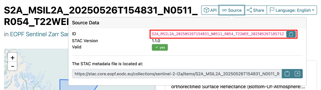
## assets, bbox, collection, geometry, id, links, properties, stac_extensions, stac_version, type

Or through the STAC catalog of the EOPF Sentinel Zarr Samples Service, on the page for that item, under “Source”:

To select a single item, supply its ID in the items() function:

example_item <- stac_source |>
  collections("sentinel-2-l2a") |>
  items("S2A_MSIL2A_20250517T085541_N0511_R064_T35QKA_20250517T112203") |>
  get_request()

example_item

## ###Item
## - id: S2A_MSIL2A_20250517T085541_N0511_R064_T35QKA_20250517T112203
## - collection: sentinel-2-l2a
## - bbox: xmin: 25.04240, ymin: 17.98988, xmax: 25.20347, ymax: 18.11305
## - datetime: 2025-05-17T08:55:41.024000Z
## - assets: 
## SR_10m, SR_20m, SR_60m, AOT_10m, B01_20m, B02_10m, B03_10m, B04_10m, B05_20m, B06_20m, B07_20m, B08_10m, B09_60m, B11_20m, B12_20m, B8A_20m, SCL_20m, TCI_10m, WVP_10m, product, product_metadata
## - item's fields: 
## assets, bbox, collection, geometry, id, links, properties, stac_extensions, stac_version, type

There are a number of helpful functions for working with an item’s assets, such as items_assets() which lists them:

# List the assets in an item
example_item |>
  items_assets()

##  [1] "SR_10m"           "SR_20m"           "SR_60m"           "AOT_10m"          "B01_20m"         
##  [6] "B02_10m"          "B03_10m"          "B04_10m"          "B05_20m"          "B06_20m"         
## [11] "B07_20m"          "B08_10m"          "B09_60m"          "B11_20m"          "B12_20m"         
## [16] "B8A_20m"          "SCL_20m"          "TCI_10m"          "WVP_10m"          "product"         
## [21] "product_metadata"

And assets_select() which allows us to select specific assets (in this case, the “Surface Reflectance - 10m” asset):

sr_10m <- example_item |>
  assets_select(asset_names = "SR_10m")

sr_10m

## ###Item
## - id: S2A_MSIL2A_20250517T085541_N0511_R064_T35QKA_20250517T112203
## - collection: sentinel-2-l2a
## - bbox: xmin: 25.04240, ymin: 17.98988, xmax: 25.20347, ymax: 18.11305
## - datetime: 2025-05-17T08:55:41.024000Z
## - assets: SR_10m
## - item's fields: 
## assets, bbox, collection, geometry, id, links, properties, stac_extensions, stac_version, type

For example, the “product” asset will be useful to working with EOPF Sample Service Zarr data, as this is the top-level Zarr hierarchy. We can select this asset, and then use assets_url() to get its URL:

example_item |>
  assets_select(asset_names = "product") |>
  assets_url()

## [1] "https://objectstore.eodc.eu:2222/e05ab01a9d56408d82ac32d69a5aae2a:202505-s02msil2a/17/products/cpm_v256/S2A_MSIL2A_20250517T085541_N0511_R064_T35QKA_20250517T112203.zarr"

It is also helpful to know which assets actually contain Zarr data. Assets can be Zarr groups, which share common dimensions and coordinates, and contain Zarr arrays within them. An asset can also be an individual Zarr array.

To look more at this, we will extract metadata attached to the Zarr assets. The "assets" entry of example_item contains a lot of useful information, but it is a bit difficult to read and manipulate:

names(example_item[["assets"]])

##  [1] "SR_10m"           "SR_20m"           "SR_60m"           "AOT_10m"          "B01_20m"         
##  [6] "B02_10m"          "B03_10m"          "B04_10m"          "B05_20m"          "B06_20m"         
## [11] "B07_20m"          "B08_10m"          "B09_60m"          "B11_20m"          "B12_20m"         
## [16] "B8A_20m"          "SCL_20m"          "TCI_10m"          "WVP_10m"          "product"         
## [21] "product_metadata"

example_item[["assets"]][["SR_10m"]]

## $gsd
## [1] 10
## 
## $href
## [1] "https://objectstore.eodc.eu:2222/e05ab01a9d56408d82ac32d69a5aae2a:202505-s02msil2a/17/products/cpm_v256/S2A_MSIL2A_20250517T085541_N0511_R064_T35QKA_20250517T112203.zarr/measurements/reflectance/r10m"
## 
## $type
## [1] "application/vnd+zarr"
## 
## $bands
## $bands[[1]]
## $bands[[1]]$name
## [1] "B02"
## 
## $bands[[1]]$common_name
## [1] "blue"
## 
## $bands[[1]]$description
## [1] "Blue (band 2)"
## 
## $bands[[1]]$center_wavelength
## [1] 0.49
## 
## $bands[[1]]$full_width_half_max
## [1] 0.098
## 
## 
## $bands[[2]]
## $bands[[2]]$name
## [1] "B03"
## 
## $bands[[2]]$common_name
## [1] "green"
## 
## $bands[[2]]$description
## [1] "Green (band 3)"
## 
## $bands[[2]]$center_wavelength
## [1] 0.56
## 
## $bands[[2]]$full_width_half_max
## [1] 0.045
## 
## 
## $bands[[3]]
## $bands[[3]]$name
## [1] "B04"
## 
## $bands[[3]]$common_name
## [1] "red"
## 
## $bands[[3]]$description
## [1] "Red (band 4)"
## 
## $bands[[3]]$center_wavelength
## [1] 0.665
## 
## $bands[[3]]$full_width_half_max
## [1] 0.038
## 
## 
## $bands[[4]]
## $bands[[4]]$name
## [1] "B08"
## 
## $bands[[4]]$common_name
## [1] "nir"
## 
## $bands[[4]]$description
## [1] "NIR 1 (band 8)"
## 
## $bands[[4]]$center_wavelength
## [1] 0.842
## 
## $bands[[4]]$full_width_half_max
## [1] 0.145
## 
## 
## 
## $roles
## [1] "data"        "reflectance" "dataset"    
## 
## $title
## [1] "Surface Reflectance - 10m"
## 
## $`xarray:open_dataset_kwargs`
## $`xarray:open_dataset_kwargs`$chunks
## named list()
## 
## $`xarray:open_dataset_kwargs`$engine
## [1] "eopf-zarr"
## 
## $`xarray:open_dataset_kwargs`$op_mode
## [1] "native"

So, we will reformat it to be easier to work with. To do so, we first load the tidyverse package for data manipulation (installing it first, if necessary):

# install.packages("tidyverse")
library(tidyverse)

We will retain only the title and roles of each asset.

asset_metadata <- example_item[["assets"]] |>
  map(\(asset) {
    asset[c("title", "roles")]
  })

head(asset_metadata, 5)

## $SR_10m
## $SR_10m$title
## [1] "Surface Reflectance - 10m"
## 
## $SR_10m$roles
## [1] "data"        "reflectance" "dataset"    
## 
## 
## $SR_20m
## $SR_20m$title
## [1] "Surface Reflectance - 20m"
## 
## $SR_20m$roles
## [1] "data"        "reflectance" "dataset"    
## 
## 
## $SR_60m
## $SR_60m$title
## [1] "Surface Reflectance - 60m"
## 
## $SR_60m$roles
## [1] "data"        "reflectance" "dataset"    
## 
## 
## $AOT_10m
## $AOT_10m$title
## [1] "Aerosol optical thickness (AOT)"
## 
## $AOT_10m$roles
## [1] "data"
## 
## 
## $B01_20m
## $B01_20m$title
## [1] "Coastal aerosol (band 1) - 20m"
## 
## $B01_20m$roles
## [1] "data"        "reflectance"

Then, we can filter to only keep assets who have the roles “dataset” (these are Zarr groups):

asset_metadata |>
  keep(\(asset) {
    "dataset" %in% asset[["roles"]]
  })

## $SR_10m
## $SR_10m$title
## [1] "Surface Reflectance - 10m"
## 
## $SR_10m$roles
## [1] "data"        "reflectance" "dataset"    
## 
## 
## $SR_20m
## $SR_20m$title
## [1] "Surface Reflectance - 20m"
## 
## $SR_20m$roles
## [1] "data"        "reflectance" "dataset"    
## 
## 
## $SR_60m
## $SR_60m$title
## [1] "Surface Reflectance - 60m"
## 
## $SR_60m$roles
## [1] "data"        "reflectance" "dataset"

Or to those who have roles “data”, but not “dataset” or “metadata” (these are individual Zarr arrays):

zarr_arrays <- asset_metadata |>
  keep(\(asset) {
    "data" %in% asset[["roles"]] & 
      !("dataset" %in% asset[["roles"]] | "metadata" %in% asset[["roles"]])
  })

names(zarr_arrays)

##  [1] "AOT_10m" "B01_20m" "B02_10m" "B03_10m" "B04_10m" "B05_20m" "B06_20m" "B07_20m" "B08_10m"
## [10] "B09_60m" "B11_20m" "B12_20m" "B8A_20m" "SCL_20m" "TCI_10m" "WVP_10m"

head(zarr_arrays, 3)

## $AOT_10m
## $AOT_10m$title
## [1] "Aerosol optical thickness (AOT)"
## 
## $AOT_10m$roles
## [1] "data"
## 
## 
## $B01_20m
## $B01_20m$title
## [1] "Coastal aerosol (band 1) - 20m"
## 
## $B01_20m$roles
## [1] "data"        "reflectance"
## 
## 
## $B02_10m
## $B02_10m$title
## [1] "Blue (band 2) - 10m"
## 
## $B02_10m$roles
## [1] "data"        "reflectance"

💪 Now it is your turn

The following expercises will help you master the STAC API and understand how to find the data you need.

Task 1: Explore Your Area of Interest

• Go to http://bboxfinder.com/ and select an area of interest (AOI) (e.g. your hometown, a research site, etc.)
• Copy the bounding box coordinates of your area of interest
• Change the provided code above to search for data over your AOI

Task 2: Temporal Analysis

• Compare data availability across different years for the Sentinel-2 L-2A Collection.
• Search for items in the year 2022
• Repeat the search for the year 2024

Task 3: Explore the SAR Mission and combine multiple criteria

• Do the same for a different Collection, the Sentinel-1 Level-1 GRD, e.g. you can use the ID sentinel-1-l1-grd
• How many assets are available for the year 2024?

Conclusion

This tutorial has provided a clear and practical introduction on how you can programmatically access and search through EOPF Sentinel Zarr Sample Service STAC API using R.

What’s next?

A tutorial on how to load an item of interest and load the Zarr data into R is coming to EOPF-101 soon! For now, please view this next tutorial in the EOPF tooling guide.